NICE TA975 (Tisagenlecleucel) HEOR Mock Case

Author

Xiaoge Zhang

Published

May 20, 2026

1 Cohort Settings & Decision Tree Parameters

Before constructing the cost-utility model, it is essential to establish the baseline characteristics of the patient cohort and the underlying spatio-temporal framework of the model. This model simulates a cohort of patients with relapsed or refractory B-cell acute lymphoblastic leukemia (R/R B-cell ALL) with an average age of 12 years and a weight of approximately 41.5 kg.

1.1 Parameter Significance

  • Baseline Characteristics: The age, sex, weight, and Body Surface Area (BSA) of the patients not only determine the setting of background mortality rates but also directly influence the costs of drug treatments measured by BSA or weight.
  • Time Horizon & Discounting: A 88-year lifetime horizon is used to fully capture the potential curative effects of CAR-T therapy. A 3.5% annual discount rate follows NICE appraisal standards to adjust the present value of future costs and health gains.
  • Decision Tree Structure: CAR-T therapy has a unique manufacturing turnaround period. During the process from apheresis to infusion, patients may discontinue due to disease progression, death, or manufacturing failure. Establishing a decision tree allows for the accurate quantification of economic expenditures and survival losses for this “Intention-to-Treat (ITT)” population during the waiting period before entering the Partitioned Survival Model (PSM) states.
Code
# ==============================================================================
# 1.1 Global Variables and Cohort Settings
# ==============================================================================

# Patient Baseline Characteristics (Base Case)
age_start <- 12 # Starting age (years)
prop_female <- 0.4304 # Proportion of female patients
avg_bsa <- 1.25 # Average Body Surface Area (m2)
avg_weight <- 41.52 # Average body weight (kg)

# Model Framework Parameters
time_horizon <- 88 # Time horizon (years)
discount_rate <- 0.035 # Annual discount rate for costs and utilities
days_in_month <- 30.4375 # Average days per month
cycle_length <- 1 # Model cycle length (1 month)

# ==============================================================================
# 1.2 Decision Tree Probabilities (Tisagenlecleucel Arm)
# ==============================================================================
1p_infusion_success <- 0.814

# Probability of discontinuing due to manufacturing failure or AEs
2p_discontinue_fail <- 0.113

# Probability of death before infusion
3p_death_pre_infusion <- 1 - (p_infusion_success + p_discontinue_fail)
1
Probability of successfully proceeding to infusion (enters PSM)
2
These patients typically switch to comparator therapies
3
Adjusted to ensure sum is 1.0 (original provided: 0.072, sum was 0.999)

2 Kaplan-Meier Curve Digitization & Pseudo-Individual Patient Data (IPD) Reconstruction

In this assessment, clinical survival coordinates were extracted with high precision from Kaplan-Meier curves using computer vision (HSV color filtering and manual anchor boundary constraints). Pseudo-IPD datasets were then reconstructed for the following 4 cohorts using the deterministic Guyot (2012) algorithm:

  1. Tisagenlecleucel arm: OS and EFS (pooled ELIANA/ENSIGN/B2101J cohort)
  2. Blinatumomab arm: OS
  3. Salvage Chemotherapy arm: OS

These reconstructed patient-level datasets serve as the foundation for the subsequent parametric survival analyses and state transition Markov/PSM models.

3 Parametric Survival Analysis & Mixture Cure Models (MCM) Fitting

Based on the core economic model settings submitted by the manufacturer, we fit Mixture Cure Models (MCM) to the pseudo-IPD using the flexsurvcure package. MCM assumes that the patient population consists of two groups: a statistically “cured” fraction (\(\theta\)) that is subject only to age-matched general population background mortality, and an “uncured” fraction (\(1 - \theta\)) whose survival follows a specific parametric distribution.

According to Document B, Table 65 “Summary of variables applied in the economic model” (Page 184) for model specifications:

  • Tisagenlecleucel (CAR-T) cohort: Both OS and EFS models are fitted using a Log-logistic mixture cure model.
  • Blinatumomab cohort: The OS model is fitted using a Log-normal mixture cure model. The EFS model does not require independent fitting, as EFS will be derived within the state-transition Markov model by applying a hazard ratio (HR) of 0.83 to the OS hazard function.
  • Salvage Chemotherapy (FLAG-IDA) cohort: The OS model is fitted using a Log-normal mixture cure model. The EFS model is also derived via HR = 0.83 and does not require independent fitting.
Code
library(survival)
library(flexsurvcure)
library(dplyr)

# 3.1 Load Reconstructed Pseudo-IPD Data
ipd_tisa_os  <- read.csv("scratch/TA975Rplct/TA975_OS_Pooled_PseudoIPD.csv")
ipd_tisa_efs <- read.csv("scratch/TA975Rplct/TA975_EFS_Pooled_PseudoIPD.csv")
ipd_blin_os  <- read.csv("scratch/TA975Rplct/Blina_Extraction/TA975_Blina_PseudoIPD.csv")
ipd_chemo_os <- read.csv("scratch/TA975Rplct/Salvage_Extraction/TA975_Salvage_PseudoIPD.csv")

# Standardize column names to uppercase (TIME, EVENT)
format_ipd <- function(df) {
  colnames(df) <- toupper(colnames(df))
  return(df)
}

ipd_tisa_os  <- format_ipd(ipd_tisa_os)
ipd_tisa_efs <- format_ipd(ipd_tisa_efs)
ipd_blin_os  <- format_ipd(ipd_blin_os)
ipd_chemo_os <- format_ipd(ipd_chemo_os)

# 3.2 Mixture Cure Model (MCM) Fitting
# If flexsurvcure fails to converge, fall back to standard parametric survival models (flexsurvreg)
fit_mcm_model <- function(df, dist, cohort_name, endpoint) {
  fit <- tryCatch({
    flexsurvcure::flexsurvcure(Surv(TIME, EVENT) ~ 1, data = df, dist = dist)
  }, error = function(e) {
    cat("Warning: flexsurvcure failed. Falling back to standard flexsurvreg.\n")
    flexsurv::flexsurvreg(Surv(TIME, EVENT) ~ 1, data = df, dist = dist)
  })
  
  return(fit)
}

# 1. Tisagenlecleucel (CAR-T) OS & EFS (Log-logistic distribution)
mcm_tisa_os  <- fit_mcm_model(ipd_tisa_os, "llogis", "Tisagenlecleucel", "OS")
mcm_tisa_efs <- fit_mcm_model(ipd_tisa_efs, "llogis", "Tisagenlecleucel", "EFS")

# 2. Blinatumomab OS (Log-normal distribution)
# EFS is derived by applying HR = 0.83 to the OS hazard function in the Markov model
mcm_blin_os  <- fit_mcm_model(ipd_blin_os, "lnorm", "Blinatumomab", "OS")

# 3. Salvage Chemotherapy OS (Log-normal distribution)
# EFS is derived by applying HR = 0.83 to the OS hazard function in the Markov model
mcm_chemo_os <- fit_mcm_model(ipd_chemo_os, "lnorm", "Salvage Chemotherapy", "OS")

# 3.3 Parameter Extraction and Summary Table for Web Presentation
get_mcm_row <- function(fit, cohort_name, endpoint, dist_name) {
  if (inherits(fit, "flexsurvcure")) {
    theta <- fit$res["theta", "est"]
    param_names <- rownames(fit$res)
    other_params <- param_names[param_names != "theta"]
    
    # Identify shape/meanlog and scale/sdlog
    p1_name <- other_params[1]
    p2_name <- other_params[2]
    p1_val <- fit$res[p1_name, "est"]
    p2_val <- fit$res[p2_name, "est"]
    
    data.frame(
      Cohort = cohort_name,
      Endpoint = endpoint,
      Model = "MCM",
      Distribution = dist_name,
      `Cure Fraction (theta)` = theta,
      `Parameter 1` = sprintf("%s = %.3f", p1_name, p1_val),
      `Parameter 2` = sprintf("%s = %.3f", p2_name, p2_val),
      check.names = FALSE
    )
  } else {
    # Standard parametric fallback
    param_names <- rownames(fit$res)
    p1_name <- param_names[1]
    p2_name <- param_names[2]
    p1_val <- fit$res[p1_name, "est"]
    p2_val <- fit$res[p2_name, "est"]
    
    data.frame(
      Cohort = cohort_name,
      Endpoint = endpoint,
      Model = "Standard Parametric",
      Distribution = dist_name,
      `Cure Fraction (theta)` = 0.0,
      `Parameter 1` = sprintf("%s = %.3f", p1_name, p1_val),
      `Parameter 2` = sprintf("%s = %.3f", p2_name, p2_val),
      check.names = FALSE
    )
  }
}

# Combine and render parameter summary
summary_df <- rbind(
  get_mcm_row(mcm_tisa_os, "Tisagenlecleucel", "OS", "Log-logistic"),
  get_mcm_row(mcm_tisa_efs, "Tisagenlecleucel", "EFS", "Log-logistic"),
  get_mcm_row(mcm_blin_os, "Blinatumomab", "OS", "Log-normal"),
  get_mcm_row(mcm_chemo_os, "Salvage Chemotherapy", "OS", "Log-normal")
)

knitr::kable(
  summary_df, 
  digits = 3, 
  caption = "Mixture Cure Model (MCM) Parameter Estimates",
  col.names = c("Cohort", "Endpoint","Model", "Distribution", "Cure Frac. (\u03b8)", "Parameter 1", "Parameter 2")
)
Mixture Cure Model (MCM) Parameter Estimates
Cohort Endpoint Model Distribution Cure Frac. (θ) Parameter 1 Parameter 2
Tisagenlecleucel OS MCM Log-logistic 0.419 shape = 1.240 scale = 17.262
Tisagenlecleucel EFS MCM Log-logistic 0.429 shape = 1.265 scale = 7.839
Blinatumomab OS MCM Log-normal 0.248 meanlog = 1.667 sdlog = 0.885
Salvage Chemotherapy OS MCM Log-normal 0.146 meanlog = 1.234 sdlog = 0.815

4 Economic Model Structure (Decision Tree & Partitioned Survival Model)

This section implements the partitioned survival model (PSM) structure and decision tree to calculate lifetime health state occupancy traces for each treatment arm.

4.1 Model Structure & Assumptions

The economic model utilizes a Partitioned Survival Model (PSM) framework consisting of three mutually exclusive health states: Event-Free Survival (EFS), Progressed Disease (PD), and Death (Dead). The state occupancy at cycle \(t\) is calculated directly from the Overall Survival (\(S_{\text{OS}}(t)\)) and Event-Free Survival (\(S_{\text{EFS}}(t)\)) functions:

  • \(\text{Prop}(\text{EFS}_t) = S_{\text{EFS}}(t)\)
  • \(\text{Prop}(\text{PD}_t) = S_{\text{OS}}(t) - S_{\text{EFS}}(t)\)
  • \(\text{Prop}(\text{Dead}_t) = 1 - S_{\text{OS}}(t)\)

The cohort starting age is 12 years. Background mortality is incorporated using a Gompertz approximation based on the England and Wales life tables. Standardised Mortality Ratio (SMR) of 4.0 is applied to the background mortality rate. Overall Survival and Event-Free Survival are constrained to never exceed the SMR-adjusted general population survival.

For Blinatumomab and Salvage Chemotherapy, EFS is derived from OS by applying a constant cumulative hazard ratio relation (\(S_{\text{EFS}} = (S_{\text{OS}})^{1/0.83}\)) for the first 5 years (60 cycles), and remains flat relative to OS thereafter: \(S_{\text{EFS}}(t) = \min(S_{\text{EFS}}(60), S_{\text{OS}}(t))\).

For the CAR-T cohort, a decision tree accounts for pre-infusion events:

  • \(P_1 = 81.4\%\) (proceeds to infusion, receiving Tisagenlecleucel survival profile)
  • \(P_2 = 11.3\%\) (discontinues before infusion, switching to 50% Blinatumomab + 50% Salvage Chemotherapy)
  • \(P_3 = 7.3\%\) (discontinues and dies at model entry, cycle = 0)

The overall Intent-to-Treat (ITT) state occupancy trace for CAR-T is calculated as:

\[ \begin{align} \mathbf{Trace}_{\text{CAR-T}}(t) &= P_1 \cdot \mathbf{Trace}_{\text{CAR-T, infused}}(t) +\\ & \qquad P_2 \cdot (0.5 \cdot \mathbf{Trace}_{\text{Blina}}(t) + 0.5 \cdot \mathbf{Trace}_{\text{Chemo}}(t)) +\\ & \qquad P_3 \cdot [0, 0, 1]^T \end{align} \]

A trapezoidal half-cycle correction is applied to state occupancies for the subsequent calculations of life years.

4.2 PSM Matrix Construction & Visualization

Code
library(ggplot2)
library(dplyr)
library(tidyr)

# 1. Initialize cycle vector: 0 to 1056 months (88 years)
cycles <- 0:1056

# 2. Define Gompertz-based background mortality and SMR multiplier functions
calc_bg_mortality_hazard <- function(t, smr = 4.0) {
  # Starting age is 12
  age <- 12 + t / 12
  
  # Gompertz approximation for England and Wales (2018-2020)
  a <- 0.00003
  b <- 0.09
  
  qx <- a * exp(b * age)
  qx <- pmin(qx, 0.99) # limit to avoid qx > 1 at extremely high age
  
  # Convert annual probability to monthly probability, then to monthly hazard
  q_monthly <- 1 - (1 - qx)^(1/12)
  h_monthly <- -log(1 - q_monthly)
  
  # Apply SMR multiplier
  return(smr * h_monthly)
}

# Pre-calculate cumulative background SMR-adjusted survival
h_bg_smr <- sapply(cycles, calc_bg_mortality_hazard)
cum_h_bg_smr <- c(0, cumsum(h_bg_smr[-length(h_bg_smr)]))
S_bg_smr <- exp(-cum_h_bg_smr)

# 3. Survival prediction function for parametric models
calc_surv_mcm <- function(t, fit, dist, is_mcm = TRUE) {
  if (t == 0) return(1.0)
  
  # Extract parameters from fit
  if (is_mcm && inherits(fit, "flexsurvcure")) {
    theta <- fit$res["theta", "est"]
    if (dist == "llogis") {
      shape <- fit$res["shape", "est"]
      scale <- fit$res["scale", "est"]
      S_u <- flexsurv::pllogis(t, shape = shape, scale = scale, lower.tail = FALSE)
    } else if (dist == "lnorm") {
      meanlog <- fit$res["meanlog", "est"]
      sdlog <- fit$res["sdlog", "est"]
      S_u <- plnorm(t, meanlog = meanlog, sdlog = sdlog, lower.tail = FALSE)
    }
    return(theta + (1 - theta) * S_u)
  } else {
    # Standard parametric model or fallback flexsurvreg
    if (dist == "llogis") {
      shape <- fit$res["shape", "est"]
      scale <- fit$res["scale", "est"]
      return(flexsurv::pllogis(t, shape = shape, scale = scale, lower.tail = FALSE))
    } else if (dist == "lnorm") {
      meanlog <- fit$res["meanlog", "est"]
      sdlog <- fit$res["sdlog", "est"]
      return(plnorm(t, meanlog = meanlog, sdlog = sdlog, lower.tail = FALSE))
    }
  }
  return(1.0)
}

# Calculate raw parametric survival for all arms
S_tisa_os_raw <- sapply(cycles, function(t) calc_surv_mcm(t, mcm_tisa_os, "llogis", is_mcm = TRUE))
S_tisa_efs_raw <- sapply(cycles, function(t) calc_surv_mcm(t, mcm_tisa_efs, "llogis", is_mcm = TRUE))
S_blin_os_raw <- sapply(cycles, function(t) calc_surv_mcm(t, mcm_blin_os, "lnorm", is_mcm = TRUE))
S_chemo_os_raw <- sapply(cycles, function(t) calc_surv_mcm(t, mcm_chemo_os, "lnorm", is_mcm = TRUE))

# 4. Generate trace matrices with constraints
build_trace <- function(S_os_raw, S_efs_raw, S_bg_smr) {
  # Constrain OS by general population SMR-adjusted survival
  S_os_constrained <- pmin(S_os_raw, S_bg_smr)
  
  # Constrain EFS to be <= OS and background survival
  S_efs_constrained <- pmin(S_efs_raw, S_os_constrained)
  
  # Compute state occupancies
  efs <- S_efs_constrained
  pd <- S_os_constrained - S_efs_constrained
  dead <- 1 - S_os_constrained
  
  data.frame(EFS = efs, PD = pd, Dead = dead)
}

# Comparator EFS derivation: S_EFS = (S_OS)^(1/0.83) for t <= 60, then flat relative to OS
derive_comparator_efs <- function(S_os_raw) {
  S_efs_derived <- numeric(length(cycles))
  for (i in seq_along(cycles)) {
    t <- cycles[i]
    if (t <= 60) {
      S_efs_derived[i] <- S_os_raw[i]^(1 / 0.83)
    } else {
      # Keep flat relative to OS after 5 years (S_EFS(t) = min(S_EFS(60), S_OS(t)))
      S_efs_derived[i] <- min(S_os_raw[61]^(1 / 0.83), S_os_raw[i])
    }
  }
  return(S_efs_derived)
}

S_blin_efs_raw <- derive_comparator_efs(S_blin_os_raw)
S_chemo_efs_raw <- derive_comparator_efs(S_chemo_os_raw)

# Build PSM traces (infused/active cohort trace)
trace_tisa_infused <- build_trace(S_tisa_os_raw, S_tisa_efs_raw, S_bg_smr)
trace_blin <- build_trace(S_blin_os_raw, S_blin_efs_raw, S_bg_smr)
trace_chemo <- build_trace(S_chemo_os_raw, S_chemo_efs_raw, S_bg_smr)

# 5. Apply ITT correction for CAR-T group
P1 <- 0.814  # Success proceed to infusion
P2 <- 0.113  # Apheresis only, switch to 50% blina + 50% chemo
P3 <- 1 - P1 - P2 # pre-infusion death (0.073)

trace_tisa_itt <- data.frame(
  EFS = P1 * trace_tisa_infused$EFS + P2 * (0.5 * trace_blin$EFS + 0.5 * trace_chemo$EFS) + P3 * 0,
  PD  = P1 * trace_tisa_infused$PD  + P2 * (0.5 * trace_blin$PD  + 0.5 * trace_chemo$PD)  + P3 * 0,
  Dead = P1 * trace_tisa_infused$Dead + P2 * (0.5 * trace_blin$Dead + 0.5 * trace_chemo$Dead) + P3 * 1.0
)

# 6. Apply Half-cycle correction (Trapezoidal Method)
apply_hcc <- function(trace) {
  n <- nrow(trace)
  trace_hcc <- trace
  
  for (col in c("EFS", "PD")) {
    val <- trace[[col]]
    val_hcc <- numeric(n)
    val_hcc[1] <- 0.5 * val[1]
    for (i in 2:n) {
      val_hcc[i] <- 0.5 * val[i] + 0.5 * val[i - 1]
    }
    trace_hcc[[col]] <- val_hcc
  }
  
  # Dead is computed as 1 - EFS - PD to ensure consistency
  trace_hcc$Dead <- 1 - trace_hcc$EFS - trace_hcc$PD
  return(trace_hcc)
}

trace_tisa_hcc <- apply_hcc(trace_tisa_itt)
trace_blin_hcc <- apply_hcc(trace_blin)
trace_chemo_hcc <- apply_hcc(trace_chemo)

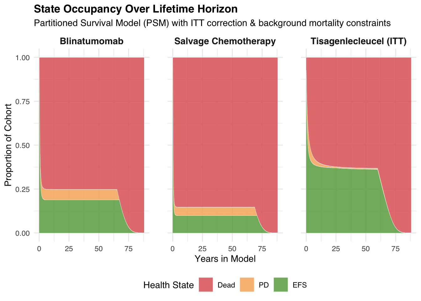
# 7. Visualization: Area plots for all three arms
prep_plot_data <- function(trace, arm_name) {
  trace %>%
    mutate(Cycle = cycles) %>%
    pivot_longer(cols = c(EFS, PD, Dead), names_to = "State", values_to = "Proportion") %>%
    mutate(
      State = factor(State, levels = c("Dead", "PD", "EFS")),
      Arm = arm_name
    )
}

plot_data <- rbind(
  prep_plot_data(trace_tisa_itt, "Tisagenlecleucel (ITT)"),
  prep_plot_data(trace_blin, "Blinatumomab"),
  prep_plot_data(trace_chemo, "Salvage Chemotherapy")
)

# Render area plot
ggplot(plot_data, aes(x = Cycle / 12, y = Proportion, fill = State)) +
  geom_area(alpha = 0.85, color = "white", size = 0.1) +
  facet_wrap(~Arm) +
  scale_fill_manual(values = c("Dead" = "#E06666", "PD" = "#F6B26B", "EFS" = "#6AA84F")) +
  labs(
    title = "State Occupancy Over Lifetime Horizon",
    subtitle = "Partitioned Survival Model (PSM) with ITT correction & background mortality constraints",
    x = "Years in Model",
    y = "Proportion of Cohort",
    fill = "Health State"
  ) +
  theme_minimal(base_family = "sans") +
  theme(
    strip.text = element_text(size = 11, face = "bold"),
    legend.position = "bottom",
    plot.title = element_text(face = "bold", size = 13),
    panel.spacing = unit(1.5, "lines")
  )

5 Health State Utilities and Adverse Event Disutilities

To evaluate the clinical benefit of each treatment strategy in terms of quality-adjusted survival, the Markov trace state occupancies are combined with health-related quality of life (HRQoL) weights. The Quality-Adjusted Life Years (QALYs) are accumulated over the cohort’s lifetime, adjusting for age-related utility decline, short-term treatment/adverse event disutility penalties, and annual discounting.

5.1 Baseline Health State Utilities & Cure Assumption

Base utilities are derived from the published literature (Kelly et al., 2015):

  • Event-Free Survival (EFS): \(U_{\text{EFS}} = 0.91\)
  • Progressed Disease / Relapsed (PD): \(U_{\text{PD}} = 0.75\)

5.1.1 Cure Assumption (Long-term Survivor Utility)

For patients surviving past 5 years (60 monthly cycles), a “cure” is assumed. Beyond this point, survivors from both EFS and PD states are assumed to achieve a long-term survivor utility of 0.91, representing a return to near-normal health state values.

5.2 Short-Term Adverse Event and Treatment Disutilities

Short-term disutilities represent acute quality of life decrements associated with treatment administration, intensive care unit (ICU) admissions, cytokine release syndrome (CRS), and subsequent allogeneic stem cell transplantation (allo-SCT). These disutilities are modeled as one-time QALY penalties subtracted in the first model cycle (Cycle 1).

The QALY decrement for any event is computed as:

\[\text{QALY Loss} = \text{Disutility Decrement} \times \left( \frac{\text{Event Duration in Days}}{365.25} \right) \times \text{Incidence}\]

5.2.1 Disutility Parameters:

  1. Base Treatment Disutility (Hospitalization): A decrement of -0.42 (based on Sung et al., 2003) is applied for the duration of treatment hospitalization:
Tisagenlecleucel Blinatumomab FLAG-IDA
25.85 days 9.24 days 21.00 days
  1. Severe CRS (ICU Stay): A decrement of -0.91 is applied for a duration of 11.10 days:
Tisagenlecleucel Blinatumomab
48.10% 5.71%
  1. Non-CRS ICU Admission (Tisagenlecleucel only): A decrement of -0.91 is applied for a duration of 1.74 days to all infused patients (100% incidence).

  2. Subsequent Stem Cell Transplant (allo-SCT): A decrement of -0.57 is applied for a duration of 365 days, weighted by the proportion of patients receiving subsequent transplant:

Tisagenlecleucel Blinatumomab FLAG-IDA
22.78% 34.29% 14.75%

5.3 Age-Adjustment and Discounting

Discounting

An annual discount rate of 3.5% is applied to both life years and QALYs, converted to a monthly discount factor:

\[\text{Discount Factor}(t) = \frac{1}{(1 + 0.035)^{t/12}}\]

5.4 Lifetime QALY Accumulation and Results

The code block below defines the utility parameters, calculates the one-time QALY losses, applies the dynamic age-adjusted utility weights, and aggregates the lifetime QALYs for the three cohorts.

Code
# 1. Parameter Definitions
u_efs_base  <- 0.91
u_pd_base   <- 0.75
u_cured     <- 0.91

# Disutility values
du_treatment <- -0.42
du_icu       <- -0.91
du_sct       <- -0.57

# Durations (days)
dur_tisa_tx  <- 25.85
dur_blin_tx  <- 9.24
dur_chemo_tx <- 21.00
dur_crs_icu  <- 11.10
dur_non_crs  <- 1.74
dur_sct      <- 365.00

# Incidences / Proportions
p_crs_tisa   <- 0.4810
p_crs_blin   <- 0.0571
p_sct_tisa   <- 0.2278
p_sct_blin   <- 0.3429
p_sct_chemo  <- 0.1475

# 2. One-Time QALY Losses in Cycle 1
calc_onetime_loss <- function(dur_tx, crs_inc = 0, crs_dur = 0, non_crs_dur = 0, sct_inc, sct_dur) {
  # All disutility terms are negative, so we subtract them from baseline (hence absolute value for loss)
  loss_tx  <- abs(du_treatment) * (dur_tx / 365.25)
  loss_crs <- abs(du_icu) * (crs_dur / 365.25) * crs_inc
  loss_non_crs <- abs(du_icu) * (non_crs_dur / 365.25)
  loss_sct <- abs(du_sct) * (sct_dur / 365.25) * sct_inc
  
  total_loss <- loss_tx + loss_crs + loss_non_crs + loss_sct
  return(total_loss)
}

# Cohort-specific one-time losses (infused/active patients)
loss_tisa_infused <- calc_onetime_loss(dur_tisa_tx, p_crs_tisa, dur_crs_icu, dur_non_crs, p_sct_tisa, dur_sct)
loss_blin_active  <- calc_onetime_loss(dur_blin_tx, p_crs_blin, dur_crs_icu, 0, p_sct_blin, dur_sct)
loss_chemo_active <- calc_onetime_loss(dur_chemo_tx, 0, 0, 0, p_sct_chemo, dur_sct)

# Intent-to-Treat (ITT) weighted loss for the CAR-T group
# P1 = 81.4% (Tisa infused), P2 = 11.3% (discontinue -> 50% Blina + 50% Chemotherapy)
loss_tisa_itt <- p_infusion_success * loss_tisa_infused + 
                 p_discontinue_fail * (0.5 * loss_blin_active + 0.5 * loss_chemo_active)

# 3. Dynamic Age-Adjustment and Baseline Utility Vector Generation
# Vectorized HSE 2014 age multipliers
get_age_multiplier <- function(age) {
  breaks <- c(-Inf, 22, 29, 34, 39, 43, 47, 50, 53, 56, 59, 62, 64, 67, 69, 71, 73, 75)
  values <- seq(1.00, 0.84, by = -0.01)
  idx <- findInterval(age, breaks, left.open = TRUE)
  ifelse(idx <= 17, values[idx], pmax(0.84 - floor((age - 75) / 2) * 0.01, 0.50))
}

# Generate age multiplier vector for all cycles (0 to 1056)
ages <- age_start + cycles / 12
age_mults <- get_age_multiplier(ages)

# Generate baseline health state utility vectors
# First 60 months: EFS = 0.91, PD = 0.75. Month 61+ (t > 60): EFS = 0.91, PD = 0.91 (Cure assumption)
ut_efs_base_vec <- rep(u_efs_base, length(cycles))
ut_pd_base_vec  <- ifelse(cycles <= 60, u_pd_base, u_cured)

# Apply age multipliers
ut_efs_vec <- ut_efs_base_vec * age_mults
ut_pd_vec  <- ut_pd_base_vec * age_mults

# 4. Lifetime QALY and Life Year Aggregation Function
calculate_outcomes <- function(trace_hcc, one_time_loss) {
  # Monthly discount factor
  df <- 1 / (1 + discount_rate)^(cycles / 12)
  
  # Life Years (LYs) accumulation (discounted and undiscounted)
  ly_undisc <- sum((trace_hcc$EFS + trace_hcc$PD) / 12)
  ly_disc   <- sum((trace_hcc$EFS + trace_hcc$PD) / 12 * df)
  
  # QALYs accumulation (discounted and undiscounted)
  qaly_cycle_undisc <- (trace_hcc$EFS * ut_efs_vec + trace_hcc$PD * ut_pd_vec) / 12
  qaly_cycle_disc   <- qaly_cycle_undisc * df
  
  qaly_undisc <- sum(qaly_cycle_undisc) - one_time_loss
  qaly_disc   <- sum(qaly_cycle_disc) - one_time_loss
  
  list(
    LYs_Undiscounted = ly_undisc,
    LYs_Discounted   = ly_disc,
    QALYs_Undiscounted = qaly_undisc,
    QALYs_Discounted   = qaly_disc
  )
}

# Calculate outcomes for each cohort
outcomes_tisa  <- calculate_outcomes(trace_tisa_hcc, loss_tisa_itt)
outcomes_blin  <- calculate_outcomes(trace_blin_hcc, loss_blin_active)
outcomes_chemo <- calculate_outcomes(trace_chemo_hcc, loss_chemo_active)

# 5. Summary Table for Web Presentation
summary_outcomes <- data.frame(
  Cohort = c("Tisagenlecleucel (ITT)", "Blinatumomab", "Salvage Chemotherapy"),
  `One-Time QALY Loss` = c(loss_tisa_itt, loss_blin_active, loss_chemo_active),
  `Undiscounted LYs` = c(outcomes_tisa$LYs_Undiscounted, outcomes_blin$LYs_Undiscounted, outcomes_chemo$LYs_Undiscounted),
  `Discounted LYs` = c(outcomes_tisa$LYs_Discounted, outcomes_blin$LYs_Discounted, outcomes_chemo$LYs_Discounted),
  `Undiscounted QALYs` = c(outcomes_tisa$QALYs_Undiscounted, outcomes_blin$QALYs_Undiscounted, outcomes_chemo$QALYs_Undiscounted),
  `Discounted QALYs` = c(outcomes_tisa$QALYs_Discounted, outcomes_blin$QALYs_Discounted, outcomes_chemo$QALYs_Discounted),
  check.names = FALSE
)

knitr::kable(
  summary_outcomes,
  digits = 4,
  caption = "Summary of Lifetime Life Years (LYs) and Quality-Adjusted Life Years (QALYs)"
)
Summary of Lifetime Life Years (LYs) and Quality-Adjusted Life Years (QALYs)
Cohort One-Time QALY Loss Undiscounted LYs Discounted LYs Undiscounted QALYs Discounted QALYs
Tisagenlecleucel (ITT) 0.1620 26.4646 10.9884 22.3716 9.4810
Blinatumomab 0.2075 17.9793 7.0687 14.9895 5.9705
Salvage Chemotherapy 0.1082 11.0436 4.2776 9.1803 3.6183

6 Costs, ICER and PAS Price Reverse Engineering

In this final section, we integrate healthcare resource costs with the clinical benefits calculated in previous steps to conduct a cost-utility analysis (CUA). We evaluate the Incremental Cost-Effectiveness Ratio (ICER) under list price, and subsequently use a root-finding algorithm to reverse-engineer the confidential Patient Access Scheme (PAS) discount price of tisagenlecleucel that aligns with official NICE decision metrics.

6.1 Cost Input Parameters and Formulation

All financial inputs are derived from the NICE TA975 appraisal documentation (Document B, Tables 65 and 43-47):

6.1.1 One-Time Initial Treatment Costs

Table 1: Initial Drug Acquisition and Hospital Service Costs
Cost Item Cohort(s) Value Description / Note
Tisagenlecleucel List Price Tisagenlecleucel £282,000.00 List price (before Patient Access Scheme discount)
NHS CAR-T Service Tariff Tisagenlecleucel £41,101.00 Covers leukapheresis, cell infusion, and early monitoring/AEs up to 100 days
Blinatumomab Treatment Cost Blinatumomab £89,436.21 Total treatment cost (drug, admin, and hospitalization)
Salvage Chemotherapy (FLAG-IDA) Salvage Chemotherapy £21,660.00 Total treatment cost (drug, admin, and hospitalization)
Table 2: Pre-treatment, Adverse Events, and Transplantation Costs
Cost Item Value Applied To / Rate Description
Bridging Chemotherapy £1,394.57 Tisagenlecleucel (pre-treatment) Non-tariff covered pre-treatment bridging therapy
Lymphodepleting Chemotherapy £404.52 Tisagenlecleucel (pre-treatment) Non-tariff covered pre-treatment lymphodepleting
Leukapheresis (uninfused only) £2,575.70 Tisagenlecleucel (uninfused) Applied only to patients discontinuing prior to infusion
Long-term AE Monitoring (IVIg) £11,176.85 Tisagenlecleucel (infused) Long-term monitoring/management for B-cell aplasia
Short-term AE Management (Blina) £2,847.49 Blinatumomab Management of short-term adverse events
Short-term AE Management (Chemo) £1,802.56 Salvage Chemotherapy Management of short-term adverse events
Subsequent allo-SCT Cost £151,227.43 Tisa: 22.78%
Blina: 34.29%
Chemo: 14.75%
Applied as a one-time cost to patients undergoing subsequent stem cell transplant

6.1.2 Monthly Health State Follow-up Costs

Cohort Health State M 1–12 M 13–24 M 25–60 M >60
Tisagenlecleucel Event-Free Survival (EFS) £472.58 £111.87 £56.18 £27.47
Progressed Disease (PD) £191.00 £263.00 £263.00 £27.47
Comparators Event-Free Survival (EFS) £263.00 £110.86 £55.43 £27.47
Progressed Disease (PD) £263.00 £263.00 £263.00 £27.47

Note: Terminal Care Cost is £13,198.42 (applied to deaths occurring within the first 5 years; for infused tisagenlecleucel, early deaths within 100 days post-infusion are covered by the NHS service tariff and therefore excluded).

6.2 ICER Calculation and PAS Price Optimization

Using the monthly half-cycle corrected state occupancies and the survival curves, we aggregate discounted lifetime costs. We then compute the baseline ICER compared to Blinatumomab and Salvage Chemotherapy.

To estimate the confidential Patient Access Scheme (PAS) discount price, we construct an objective function: \[\text{ICER}_{\text{Tisa vs Blina}}(\text{Price}_{\text{PAS}}) - £19,218 = 0\] Using R’s uniroot function, we search the interval \([0, 282000]\) to solve for the PAS price.

Code
# 1. Parameter Definitions
price_tisa_list    <- 282000.00
tariff_nhs         <- 41101.00
c_bridging         <- 1394.57
c_lymphodepleting  <- 404.52
c_leukapheresis    <- 2575.70
c_ivig             <- 11176.85
c_sct              <- 151227.43
c_terminal_care    <- 13198.42

c_treatment_blin   <- 89436.21
c_treatment_chemo  <- 21660.00
c_ae_blin          <- 2847.49
c_ae_chemo         <- 1802.56

p_infusion_success   <- 0.814
p_discontinue_fail   <- 0.113
p_pre_infusion_death <- 0.073

p_sct_tisa         <- 0.2278
p_sct_blin         <- 0.3429
p_sct_chemo        <- 0.1475

# 2. Monthly Follow-up Cost Vector Construction
cost_tisa_efs <- dplyr::case_when(
  cycles <= 12 ~ 472.58,
  cycles <= 24 ~ 111.87,
  cycles <= 60 ~ 56.18,
  TRUE ~ 27.47
)

cost_tisa_pd <- dplyr::case_when(
  cycles <= 12 ~ 191.00,
  cycles <= 60 ~ 263.00,
  TRUE ~ 27.47
)

cost_comp_efs <- dplyr::case_when(
  cycles <= 12 ~ 263.00,
  cycles <= 24 ~ 110.86,
  cycles <= 60 ~ 55.43,
  TRUE ~ 27.47
)

cost_comp_pd <- dplyr::case_when(
  cycles <= 60 ~ 263.00,
  TRUE ~ 27.47
)

# 3. Terminal Care Cost Vector Calculation
calc_terminal_care_cost <- function(trace, is_tisa = FALSE) {
  dying <- numeric(length(cycles))
  dying[1] <- 0
  for (i in 2:length(cycles)) {
    dying[i] <- (trace$EFS[i-1] + trace$PD[i-1]) - (trace$EFS[i] + trace$PD[i])
  }
  
  tc_cost <- numeric(length(cycles))
  for (i in 1:length(cycles)) {
    t <- cycles[i]
    if (t <= 60) {
      if (is_tisa && t <= 3) {
        tc_cost[i] <- 0 # Covered under CAR-T NHS tariff
      } else {
        tc_cost[i] <- dying[i] * c_terminal_care
      }
    } else {
      tc_cost[i] <- 0
    }
  }
  return(tc_cost)
}

discount_rate <- 0.035
df <- 1 / (1 + discount_rate)^(cycles / 12)

# 4. Total Discounted Cost Calculation for Comparators
# Blinatumomab total cost
trace_blin_hcc <- apply_hcc(trace_blin)
followup_cost_blin <- sum((trace_blin_hcc$EFS * cost_comp_efs + trace_blin_hcc$PD * cost_comp_pd) * df)
tc_cost_blin <- sum(calc_terminal_care_cost(trace_blin, is_tisa = FALSE) * df)
one_time_cost_blin <- c_treatment_blin + c_ae_blin + p_sct_blin * c_sct
total_cost_blin <- one_time_cost_blin + followup_cost_blin + tc_cost_blin

# Salvage Chemotherapy total cost
trace_chemo_hcc <- apply_hcc(trace_chemo)
followup_cost_chemo <- sum((trace_chemo_hcc$EFS * cost_comp_efs + trace_chemo_hcc$PD * cost_comp_pd) * df)
tc_cost_chemo <- sum(calc_terminal_care_cost(trace_chemo, is_tisa = FALSE) * df)
one_time_cost_chemo <- c_treatment_chemo + c_ae_chemo + p_sct_chemo * c_sct
total_cost_chemo <- one_time_cost_chemo + followup_cost_chemo + tc_cost_chemo

# 5. Tisagenlecleucel Cost Functions
# Infused cohort total cost (dependent on price)
trace_tisa_infused_hcc <- apply_hcc(trace_tisa_infused)
followup_cost_tisa_infused <- sum((trace_tisa_infused_hcc$EFS * cost_tisa_efs + trace_tisa_infused_hcc$PD * cost_tisa_pd) * df)
tc_cost_tisa_infused <- sum(calc_terminal_care_cost(trace_tisa_infused, is_tisa = TRUE) * df)

total_cost_tisa_infused <- function(price) {
  one_time <- price + tariff_nhs + c_bridging + 0.96 * c_lymphodepleting + c_ivig + p_sct_tisa * c_sct
  return(one_time + followup_cost_tisa_infused + tc_cost_tisa_infused)
}

# Pre-treatment cost for discontinued and pre-infusion death cohorts
c_pre_tx <- c_leukapheresis + 0.5 * c_bridging + 0.5 * c_lymphodepleting

# ITT cohort total cost (dependent on price)
total_cost_tisa_itt <- function(price) {
  cost_p1 <- p_infusion_success * total_cost_tisa_infused(price)
  cost_p2 <- p_discontinue_fail * (c_pre_tx + 0.5 * total_cost_blin + 0.5 * total_cost_chemo)
  cost_p3 <- p_pre_infusion_death * (c_pre_tx + c_terminal_care)
  return(cost_p1 + cost_p2 + cost_p3)
}

# 6. Baseline Cost-Utility Analysis under List Price
cost_tisa_list <- total_cost_tisa_itt(price_tisa_list)

qaly_tisa  <- outcomes_tisa$QALYs_Discounted
qaly_blin  <- outcomes_blin$QALYs_Discounted
qaly_chemo <- outcomes_chemo$QALYs_Discounted

# Incremental calculations
inc_qaly_blin  <- qaly_tisa - qaly_blin
inc_qaly_chemo <- qaly_tisa - qaly_chemo

inc_cost_blin_list  <- cost_tisa_list - total_cost_blin
inc_cost_chemo_list <- cost_tisa_list - total_cost_chemo

icer_blin_list  <- inc_cost_blin_list / inc_qaly_blin
icer_chemo_list <- inc_cost_chemo_list / inc_qaly_chemo

# 7. Patient Access Scheme (PAS) Discount Price Search
# Objective function: ICER vs Blina = 19218
obj_fun <- function(price) {
  cost_tisa <- total_cost_tisa_itt(price)
  icer <- (cost_tisa - total_cost_blin) / inc_qaly_blin
  return(icer - 19218.0)
}

sol <- uniroot(obj_fun, interval = c(0, price_tisa_list))
pas_price <- sol$root
discount_pct <- (1 - pas_price / price_tisa_list) * 100

# 8. Re-evaluation under PAS Discount Price
cost_tisa_pas <- total_cost_tisa_itt(pas_price)
inc_cost_blin_pas  <- cost_tisa_pas - total_cost_blin
inc_cost_chemo_pas <- cost_tisa_pas - total_cost_chemo

icer_blin_pas  <- inc_cost_blin_pas / inc_qaly_blin
icer_chemo_pas <- inc_cost_chemo_pas / inc_qaly_chemo

# 9. Results Table Compilation
summary_list <- data.frame(
  Cohort = c("Tisagenlecleucel (ITT)", "Blinatumomab", "Salvage Chemotherapy"),
  `Total Cost` = c(cost_tisa_list, total_cost_blin, total_cost_chemo),
  `Total QALYs` = c(qaly_tisa, qaly_blin, qaly_chemo),
  `Incremental Cost` = c(NA, inc_cost_blin_list, inc_cost_chemo_list),
  `Incremental QALYs` = c(NA, inc_qaly_blin, inc_qaly_chemo),
  `ICER (£/QALY)` = c(NA, icer_blin_list, icer_chemo_list),
  check.names = FALSE
)

summary_pas <- data.frame(
  Cohort = c("Tisagenlecleucel (ITT)", "Blinatumomab", "Salvage Chemotherapy"),
  `Total Cost` = c(cost_tisa_pas, total_cost_blin, total_cost_chemo),
  `Total QALYs` = c(qaly_tisa, qaly_blin, qaly_chemo),
  `Incremental Cost` = c(NA, inc_cost_blin_pas, inc_cost_chemo_pas),
  `Incremental QALYs` = c(NA, inc_qaly_blin, inc_qaly_chemo),
  `ICER (£/QALY)` = c(NA, icer_blin_pas, icer_chemo_pas),
  check.names = FALSE
)

6.3 Cost-Utility Results

CUA under List Price (£282,000)

The table below shows the cost-effectiveness results under the list price of tisagenlecleucel.

Code
knitr::kable(
  summary_list,
  digits = 2,
  caption = "Cost-Utility Analysis Results under List Price (Discounted at 3.5%)"
)
Table 1: Cost-Utility Analysis Results under List Price (Discounted at 3.5%)
Cohort Total Cost Total QALYs Incremental Cost Incremental QALYs ICER (£/QALY)
Tisagenlecleucel (ITT) 328517.65 9.48 NA NA NA
Blinatumomab 159086.18 5.97 169431.5 3.51 48265.34
Salvage Chemotherapy 60372.27 3.62 268145.4 5.86 45737.62

Reverse-Engineered PAS Price and CUA Results

Through root-finding optimization, the estimated PAS price for tisagenlecleucel is calculated.

Table 2: Summary of Reverse-Engineered Patient Access Scheme (PAS) Price
Metric Value
List Price 282000.00
PAS Price 156731.85
Absolute Discount (£) 125268.15
PAS Discount Percentage (%) 44.42

The table below shows the cost-effectiveness results under the estimated PAS price.

Code
knitr::kable(
  summary_pas,
  digits = 2,
  caption = "Cost-Utility Analysis Results under PAS Price (Discounted at 3.5%)"
)
Table 3: Cost-Utility Analysis Results under PAS Price (Discounted at 3.5%)
Cohort Total Cost Total QALYs Incremental Cost Incremental QALYs ICER (£/QALY)
Tisagenlecleucel (ITT) 226549.38 9.48 NA NA NA
Blinatumomab 159086.18 5.97 67463.19 3.51 19218.00
Salvage Chemotherapy 60372.27 3.62 166177.11 5.86 28344.87