TA1092 EAG Appraisal Case: Pembrolizumab + Chemotherapy in Endometrial Cancer

Survival Extrapolation, Subgroup Uncertainty, and the EAG Review Lens

ImportantMock Case Disclosure

This is a methodological proof-of-concept. All context and data are generated or reconstructed for demonstration purposes. Patient-level data are pseudo-individual patient data (pseudo-IPD) reconstructed from published trial curves (KEYNOTE-868) using digitization and the Guyot algorithm. All numbers, economic models, and clinical parameters are illustrative only and do not represent the proprietary or confidential manufacturer model submission.

1 Background

NoteConsulting Blueprint: Value-Driven Scope & Budget Control (Click to expand)

This case study functions as a high-fidelity HTA appraisal audit and model reconstruction portfolio, simulating the role of a Principal Health Economist or Senior Modeler in a consulting practice. It evaluates the NICE technology appraisal TA1092 concerning pembrolizumab with carboplatin and paclitaxel for first-line advanced or recurrent endometrial cancer.

In commercial HEOR consulting, project delivery is strictly constrained by billable hours and the contract’s Scope of Work (SOW). A common challenge for modelers transitioning from academia is the tendency toward academic perfectionism—spending excessive hours pursuing non-reproducible parameters or trying to replicate confidential manufacturer calculations.

This project demonstrates a pragmatic, value-driven scope management strategy under a target budget. To show compliance with commercial constraints and resource allocation, the relative effort distribution for each technical step is logged in the page margins (as percentages of total project effort). The objective is not to reproduce the confidential manufacturer workbook or match the exact confidential ICERs (which are driven by undisclosed discounts). Instead, we deliberately restrict our scope to focus on high-value technical nodes—the key structural assumptions and parameters that EAGs challenge most and to which the cost-effectiveness decisions are highly sensitive.

Project Scope Statement

Domain	In Scope (High-Value Delivery)	Out of Scope (Academic perfectionism / Confidentiality barriers)
Efficacy Data	• Reconstructing pseudo-IPD from published trial subgroup curves (NEJM Fig 2A/B) via computer vision (HSV) and Guyot-reconstructed KM estimates. • Fitting candidate parametric distributions and Royston-Parmar splines in R.	• Full patient-level clinical trial database replication (confidential and unavailable).
Model Structure	• Building a de novo 3-state weekly PSM simulation engine in R (progression-free, progressed disease, death).	• Replicating the exact proprietary, multi-sheet manufacturer Excel workbook layout.
HTA Adjustments	• Coding technical solutions for HTA critiques: starting age corrections, treatment-effect waning (5–7 years), and curve-crossing capping (pmin(PFS, OS)).	• Re-estimating utilities or resource frequencies without public data access.
Costs & Economics	• Mapping public list prices, administration costs, acute AE management costs, and NHS-aligned subsequent therapies.	• Accessing or estimating confidential Drug Access Agreements (patient access scheme discounts).
Uncertainty Analysis	• Running parallel deterministic scenario analysis (Company vs. EAG base case) and parameter capping checks.	• Full 5,000-run probabilistic sensitivity analysis (PSA) requiring joint parameter covariance matrices.

1.1 Clinical Context

This page presents a de novo economic evaluation and survival extrapolation audit reconstructing the NICE TA1092 appraisal of pembrolizumab in combination with chemotherapy for first-line advanced or recurrent endometrial cancer. The analysis replicates the clinical and economic modeling choices debated during the technology appraisal consultations, contrasting standard parametric modeling against the flexible spline-based models preferred by the External Assessment Group (EAG). By leveraging digitized patient-level data, the model explores the cost-effectiveness impact of structural and parameter uncertainties across molecularly defined subgroups (dMMR and pMMR).

The clinical and decision framework is structured as follows:

• Disease Area: Untreated primary advanced or recurrent endometrial cancer.
• Intervention: Pembrolizumab in combination with carboplatin and paclitaxel, followed by pembrolizumab monotherapy maintenance (for up to 14 additional cycles).
• Comparator: Carboplatin and paclitaxel followed by placebo maintenance (representing the KEYNOTE-868 clinical trial setting) and carboplatin/paclitaxel alone without maintenance (representing standard NHS clinical practice).
• Key Clinical Trial: KEYNOTE-868 / NRG-GY018, which evaluated the efficacy and safety of the combination.
• Main Modeling Challenge: The combination of immunotherapy and platinum-taxane chemotherapy requires translating immature trial overall survival (OS) data into long-term projections. The key clinical and economic question is whether the additional cost of pembrolizumab is justified by the progression-free survival (PFS) and OS gains, particularly when long-term efficacy waning and structural curve-crossing constraints are applied.

1.2 Decision Problem

Element	Working abstraction
Population	Adults with untreated primary advanced or recurrent endometrial cancer
Subgroups	dMMR/MSI-H and pMMR/MSS populations
Intervention	Pembrolizumab + carboplatin + paclitaxel, then pembrolizumab maintenance
Comparator	Carboplatin + paclitaxel followed by placebo maintenance (trial); Carboplatin + paclitaxel alone without maintenance (NHS economic model)
Outcomes	PFS, OS, adverse events, health-related quality of life, costs, QALYs
Model type	Three-state PSM
NICE decision tension	Whether extrapolated survival benefit is clinically plausible and cost-effective across molecular subgroups

1.3 Evidence & Appraisal Registry

To maintain a concise background narrative, the complete HTA literature registry and parameter traceability mapping are detailed in the HTA Evidence & Reference Registry in the Appendix.

NoteModeler’s Initial Risk Screening & HTA Audit Focus (Click to expand)

When evaluating a manufacturer’s cost-effectiveness submission for an oncology immunotherapy combination, an experienced HTA model auditor screens for standard systemic risk nodes. In this appraisal, our initial risk-screening checklist targets four critical domains:

1. Survival Extrapolation & Tail Plausibility (High Risk):
   • Audit Target: When clinical trial follow-up is relatively short (median < 2 years), the choice of parametric models is highly sensitive. We must verify if the long-term overall survival (OS) tails are clinically plausible or if they project unrealistic lifetime “immortal patient” fractions.
   • Key Focus: Subgroup sample sizes (dMMR vs. pMMR) and the risk of PFS and OS curves crossing in the long term, which violates logical consistency.
2. Immunotherapy Treatment Duration & Efficacy Waning (High Risk):
   • Audit Target: Immunotherapies like pembrolizumab are typically capped (e.g., a 2-year stopping rule). The model must not assume that treatment benefit persists indefinitely after treatment discontinuation.
   • Key Focus: Implementing and testing treatment-effect waning scenarios (e.g., waning starting at 2 or 5 years and converging to control hazards) to evaluate the stability of the ICER.
3. Subgroup Applicability & Data Maturity (Medium Risk):
   • Audit Target: The clinical and economic benefits may differ significantly between mismatch repair deficient (dMMR) and proficient (pMMR) cohorts. We need to check if separate models are statistically stable and if baseline characteristics align with the UK target population.
4. Resource Cost & Subsequent Therapy Alignments (Medium Risk):
   • Audit Target: Subsequent treatment mixes in the comparator arm must reflect real-world NHS standard pathways rather than non-reimbursed trial settings, as differences in active subsequent therapies can distort the cost delta.

2 EAG Critique Lens

2.1 How the EAG Reviews This Type of Case

The EAG is not only checking whether the model runs. It is asking whether the company’s assumptions are:

• internally consistent with trial evidence;
• externally plausible against clinical knowledge;
• aligned with NHS treatment pathways;
• transparent enough for committee decision-making;
• conservative enough when evidence is immature.

This distinction is important for the portfolio: a health economist in consulting must be able to understand both the company logic and the EAG logic.

2.2 Summary of NICE Decision Tensions

Based on the HTA dossier review, the appraisal debate centers on translating immature trial survival data into a 30-year extrapolation model. The key methodological debates include:

• Survival Tail Plausibility: Standard parametric models preferred by the company yielded optimistic long-term tails. The EAG preferred flexible spline models to better capture hazard dynamics.
• Curve-Crossing Implausibility: The EAG’s spline-based placebo PFS model crossed and exceeded the active pembrolizumab PFS model in the long-term tail. This logical inconsistency required a structural capping mechanism.
• Efficacy Waning: The company assumed infinite treatment benefit post-discontinuation, which the EAG challenged. A compromise waning window was introduced to transition active treatment hazards to control hazards.
• Utility Consistency: To avoid confounding utility estimates by mixing clinical trial sources (KEYNOTE-158 and KEYNOTE-B21), the EAG advocated for exclusive use of KEYNOTE-158.

2.3 Summary of the 10 EAG Key Issues

The EAG identified ten key clinical, methodological, and economic issues in the company’s submission. To demonstrate compliance with a value-driven consulting scope (where we avoid duplicating every minor manufacturer calculation), this case study focuses on auditing and simulating the two most critical methodological and structural issues: Issue 3 (Short trial follow-up / data immaturity) and Issue 5 (Uncertain overall survival benefit). These two issues represent the primary sources of uncertainty in long-term extrapolation and have the most significant impact on the resulting cost-effectiveness decisions.

The complete list of the ten key issues is summarized below, with links to the interactive audit sections for the two prioritized issues:

1. Representativeness of post-hoc all-comer analysis: Post-hoc pooling of trial cohorts may not represent the trial’s original design and statistical analysis plan.
2. Subgroup limitations: Site of recurrence (local vs. metastatic) and debulking surgery history were not systematically collected in KEYNOTE-868.
3. Short trial follow-up (Data Immaturity): Immaturity of trial data limits the robustness of long-term survival effectiveness conclusions.
4. Subgroup-restricted HRQoL: Health-related quality of life was collected only in the pMMR cohort, leaving the dMMR cohort without trial-specific utility data.
5. Uncertain overall survival benefit: The company’s survival models potentially overestimate long-term immunotherapy tail benefits.
6. Understated baseline age: The modeled baseline age (65.4 years) was younger than standard UK patients (67.1 years), affecting background mortality.
7. Representativeness of health state utilities: Mapped utilities from KEYNOTE-158 (second-line dMMR) may not represent the first-line all-comer population.
8. Underestimated safety monitoring resources: Safety monitoring costs (blood, liver, thyroid tests) for patients on active immunotherapy were omitted.
9. Incomplete adverse event costing: High >=5% incidence threshold omitted expensive immunotherapy-related adverse events.
10. Misaligned subsequent treatment mix: Subsequent therapies in the comparator arm did not align with NHS clinical guidelines.

2.4 EAG Challenge Log

Click to expand: Detailed EAG Challenge Log & ICER Impact Map

Issue	Company position	EAG concern	Why the EAG cares	Potential ICER direction
OS extrapolation	Standard parametric curves (log-logistic/gamma) based on trial data fit	Overestimated overall survival tails due to short trial follow-up; preferred flexible splines for pMMR	Long-term OS tail is the major driver of lifetime QALY gains	Significantly increases the ICER
PFS extrapolation	Generalised gamma (dMMR) and 2-piece generalised gamma (pMMR)	Prone to tail overestimation; preferred log-logistic/generalised gamma (dMMR) and flexible splines (pMMR)	Determines duration of progression-free utility and active treatment exposure	Increases the ICER
Curve crossing	Long-term crossing is clinically implausible; active treatment should always be superior	Crossing is a tail extrapolation uncertainty artifact and doesn’t invalidate observed trial fit	PFS must not cross treatment arms; uncapped models are structurally flawed	Modestly reduces the ICER when placebo PFS is capped
Subgroup modelling	Modeled dMMR and pMMR cohorts separately using trial subgroup baseline inputs	Supported separate models, but highlighted dMMR immaturity due to small sample size	Treatment effect and background risks differ fundamentally by molecular status	Results in distinct ICERs for dMMR (cost-effective) and pMMR (marginal)
Treatment effect waning	No waning applied (assumed lifetime immunotherapy benefit)	Short trial follow-up cannot justify indefinite post-discontinuation benefit; preferred 5-7 year waning	Overestimates long-term survival gain in the extrapolated tail	Significantly increases the ICER
Utility values	Used mixed sources (KEYNOTE-158 for PD, KEYNOTE-B21 for PF health states)	Opposed mixing utility sources; preferred using KEYNOTE-158 exclusively for all states	Health state utility values directly scale cumulative QALY gains	Modestly to significantly increases the ICER
Starting age	65.4 years (mean age of dMMR/pMMR pooled cohort in KEYNOTE-868)	Trial population is younger than UK real-world patients (mean age 67.1 years based on Pennington 2016)	Affects background mortality and lifetime QALY potential	Modestly increases ICER (due to higher background mortality truncating long-term QALYs)
Resource use / Monitoring	Standard monitoring costs applied to both arms	Intervention arm requires additional routine safety monitoring (blood tests, thyroid, liver, glucose tests)	Underestimating routine monitoring costs artificially reduces intervention costs	Modestly increases ICER (due to higher treatment monitoring costs in the intervention arm)
Adverse events	Standard AE costing (Grade 3-5 AEs with >5% incidence; only anemia/hypertension costed)	Immunotherapy-related AEs (irAEs) are expensive and omitted from the costings	Omiting severe immunotherapy AEs understates treatment-related management costs	Minimally increases ICER (due to limited impact of one-off acute AE costs)
Subsequent therapy	Company assumed a portion of the CT arm receives pembrolizumab monotherapy post-progression	Pembrolizumab monotherapy is not NHS standard 2L care for pMMR patients; should be pembrolizumab + lenvatinib	Standardizing subsequent care in the comparator arm directly influences comparator cost levels	Decreases ICER (due to subsequent therapy costs in the comparator arm narrowing the cost delta)

2.5 Committee Preferred Assumptions

Click to expand: Company vs. EAG vs. Committee Preferred Assumptions Table

Assumption	Company base case	EAG preferred	Committee preferred	My comment
dMMR OS curve	Log-logistic (pembro) / Exponential (placebo)	Log-logistic (pembro) / Exponential (placebo)	Log-logistic (pembro) / Exponential (placebo)	Consensus reached. Both parties agreed these represented the best fit and clinical plausibility for the dMMR cohort.
pMMR OS curve	Log-logistic (pembro) / Gamma (placebo)	1-knot normal spline (pembro) / 1-knot hazard spline (placebo)	1-knot normal spline (pembro) / 1-knot hazard spline (placebo)	Committee preferred the EAG’s spline models to capture the changing hazard observed in the trial.
dMMR PFS curve	Generalised gamma (pembro) / 2-piece gamma (placebo, 27-wk cut)	Log-logistic (pembro) / Generalised gamma (placebo)	Log-logistic (pembro) / Generalised gamma (placebo)	Committee adopted the EAG’s preferred curves due to improved fit and tail plausibility.
pMMR PFS curve	2-piece generalised gamma (pembro, 37-wk cut) / 1-knot odds spline (placebo)	1-knot hazard spline (pembro) / 2-knot hazard spline (placebo)	1-knot hazard spline (pembro) / 2-knot hazard spline (placebo, capped)	Sided with the company’s implausibility argument: mandated capping placebo PFS at pembro PFS in the tail.
Waning assumption	No waning (lifetime treatment effect)	Gradual waning 5 to 7 years (all patients)	Gradual waning 5 to 7 years (non-complete responders only)	Plausible compromise. Waning applied between 5-7 years only for patients without complete response.
Utility source	Mixed (KEYNOTE-158 for PD, KEYNOTE-B21 for PF)	KEYNOTE-158 (all states and subgroups)	KEYNOTE-158 (all states and subgroups)	Committee preferred keeping a single consistent trial source to avoid mixing different patient populations.
Starting age	65.4 years	67.1 years	67.1 years	Committee preferred 67.1 years to reflect real-world NHS patients and maintain consistency with TA963
Resource use / Monitoring	Standard monitoring	Additional routine safety monitoring (EAG clinical expert estimates)	Additional routine safety monitoring	Committee preferred EAG’s monitoring frequencies to reflect NHS clinical guidelines for patients on immunotherapy
Adverse events	>5% Grade 3-5 AEs (anemia & hypertension only)	Include Grade 3-5 AEs with >=2% incidence	Company base case (>5% Grade 3-5 AEs)	Committee accepted the company base case because including broader AEs had a minimal impact on the ICER
Subsequent therapy	Pembrolizumab monotherapy allowed in CT arm	Reallocate pembrolizumab monotherapy to pembrolizumab + lenvatinib	Reallocated subsequent therapy for pMMR patients	Committee preferred aligning subsequent therapies with NHS clinical guidelines for pMMR patients, which reduced the cost delta and decreased the ICER

3 Workflow Setup & Exploratory Analysis

Effort Allocation: 15%

• Extracted subgroup curves using Computer Vision HSV color segmentation.
• Reconstructed pseudo-IPD using the Guyot algorithm.

This section initializes the analysis environment and loads the raw clinical inputs. The individual patient-level data (IPD) used throughout this appraisal were reconstructed from the published Kaplan-Meier survival curves in the KEYNOTE-868 (NRG-GY018) trial (Eskander et al., 2023).

The reconstruction workflow follows a standardized HTA auditing process:

1. Digitization: Time-survival coordinates were extracted from the published PFS and OS curves for the mismatch repair deficient (dMMR) and mismatch repair proficient (pMMR) cohorts using a custom computer vision HSV (Hue, Saturation, Value) color segmentation script, which eliminates the manual error associated with point-and-click tools.
2. IPD Re-creation: The digital coordinates, along with reported patients-at-risk tables and event counts, were processed using the iterative algorithm proposed by Guyot et al. (2012) to reconstruct patient-level times and censoring indicators.
3. Harmonization: The individual datasets for each endpoint, subgroup, and treatment arm were consolidated into a single long-format database (survival_ipd_long.csv).
4. Validation: The reconstructed individual patient data (pseudo-IPD) are summarized and plotted below to confirm structural alignment with the original trial publications prior to fitting parametric survival models.

library(survival)
library(flexsurv)
library(dplyr)
library(tidyr)
library(purrr)
library(readr)
library(ggplot2)
library(knitr)

# Set file paths
base_dir <- normalizePath(".", mustWork = TRUE)
input_path <- file.path(base_dir, "survival_inputs", "survival_ipd_long.csv")
output_dir <- file.path(base_dir, "survival_models")
plot_dir <- file.path(output_dir, "plots")

dir.create(output_dir, showWarnings = FALSE, recursive = TRUE)
dir.create(plot_dir, showWarnings = FALSE, recursive = TRUE)

# Load and transform reconstructed IPD
ipd <- read_csv(input_path, show_col_types = FALSE) |>
  mutate(
    subgroup = factor(subgroup, levels = c("dMMR", "pMMR")),
    endpoint = factor(endpoint, levels = c("PFS", "OS")),
    treatment = factor(treatment, levels = c("placebo_chemo", "pembro_chemo")),
    status = as.integer(status),
    time_months = as.numeric(time_months),
    curve_id = paste(subgroup, endpoint, treatment, sep = "_")
  )

# Validation subset for standard parametric testing
pmmr_pfs_pembro_ipd <- ipd |>
  filter(subgroup == "pMMR", endpoint == "PFS", treatment == "pembro_chemo")

# Reconstructed Kaplan-Meier Curves (Total N = `r nrow(ipd)`)
km_data <- ipd |>
  mutate(
    treatment_label = ifelse(treatment == "pembro_chemo", "Pembrolizumab + Chemo", "Placebo + Chemo")
  ) |>
  group_by(subgroup, endpoint, treatment_label) |>
  group_modify(~{
    fit <- survfit(Surv(time_months, status) ~ 1, data = .x)
    tibble(
      time_months = c(0, fit$time),
      survival = c(1, fit$surv)
    )
  }) |>
  ungroup()

ggplot(km_data, aes(x = time_months, y = survival, color = treatment_label)) +
  geom_step(linewidth = 0.8) +
  facet_grid(endpoint ~ subgroup) +
  scale_y_continuous(limits = c(0, 1), breaks = seq(0, 1, 0.2)) +
  scale_color_manual(values = c("Placebo + Chemo" = "#E69F00", "Pembrolizumab + Chemo" = "#0072B2")) +
  labs(
    title = "Reconstructed Kaplan-Meier Curves",
    subtitle = "Faceted by Endpoint (PFS/OS) and Subgroup (dMMR/pMMR) from KEYNOTE-868",
    x = "Months",
    y = "Survival Probability",
    color = "Treatment Arm"
  ) +
  theme_minimal() +
  theme(
    legend.position = "bottom",
    strip.text = element_text(face = "bold", size = 10),
    plot.title = element_text(face = "bold", size = 12)
  )

4 Parametric Survival Fitting & Diagnostics

Effort Allocation: 30%

• Developed automated fitting wrapper for batch survival modeling.
• Evaluated AIC/BIC goodness-of-fit criteria across 56 model configurations.

This section implements the standard parametric survival analysis. We fit seven candidate distributions (exponential, Weibull, Gompertz, log-normal, log-logistic, gamma, and generalized gamma) to each of the eight reconstructed patient-level survival curves (PFS and OS for dMMR and pMMR cohorts under both active pembrolizumab and placebo comparator arms).

Goodness-of-fit within the observed trial period is evaluated using standard information criteria (Akaike Information Criterion, AIC, and Bayesian Information Criterion, BIC) to establish a first-pass statistical baseline for survival modeling.

# Define candidate distributions for flexsurv
candidate_dists <- c(
  "exponential" = "exp",
  "weibull" = "weibull",
  "gompertz" = "gompertz",
  "lognormal" = "lnorm",
  "loglogistic" = "llogis",
  "gamma" = "gamma",
  "generalized_gamma" = "gengamma"
)

# Define safe fitting wrapper
`%||%` <- function(x, y) if (is.null(x)) y else x

fit_one_distribution <- function(dat, dist_label, dist_name) {
  tryCatch(
    {
      fit <- flexsurvreg(Surv(time_months, status) ~ 1, data = dat, dist = dist_name)
      n_par <- nrow(fit$res)
      fit_aic <- as.numeric(fit$AIC %||% NA_real_)
      fit_loglik <- as.numeric(fit$loglik %||% NA_real_)

      tibble(
        dist_label = dist_label,
        dist_name = dist_name,
        fit = list(fit),
        converged = TRUE,
        error = NA_character_,
        aic = fit_aic,
        bic = -2 * fit_loglik + log(nrow(dat)) * n_par,
        loglik = fit_loglik,
        n = nrow(dat),
        events = sum(dat$status)
      )
    },
    error = function(e) {
      tibble(
        dist_label = dist_label,
        dist_name = dist_name,
        fit = list(NULL),
        converged = FALSE,
        error = conditionMessage(e),
        aic = NA_real_,
        bic = NA_real_,
        loglik = NA_real_,
        n = nrow(dat),
        events = sum(dat$status)
      )
    }
  )
}

# Run batch fitting across all curves
curve_groups <- ipd |>
  group_by(subgroup, endpoint, treatment, arm_role, treatment_label, curve_id) |>
  group_split()

fit_tbl <- map_dfr(curve_groups, function(dat) {
  meta <- dat |>
    slice(1) |>
    select(subgroup, endpoint, treatment, arm_role, treatment_label, curve_id)

  res <- map2_dfr(
    names(candidate_dists),
    candidate_dists,
    ~fit_one_distribution(dat, .x, .y)
  )

  bind_cols(res, meta[rep(1, nrow(res)), ])
})

# Extract parameter estimates for downstream modeling
extract_parameters <- function(fit) {
  if (is.null(fit)) {
    return(tibble(parameter = character(), estimate = numeric(), se = numeric()))
  }
  as.data.frame(fit$res) |>
    tibble::rownames_to_column("parameter") |>
    as_tibble() |>
    transmute(parameter, estimate = est, se = se)
}

parameter_tbl <- fit_tbl |>
  filter(converged) |>
  mutate(parameters = map(fit, extract_parameters)) |>
  select(subgroup, endpoint, treatment, curve_id, dist_label, parameters) |>
  unnest(parameters)

# Select first-pass statistical best fits (minimum AIC)
best_fits <- fit_tbl |>
  filter(converged, !is.na(aic)) |>
  group_by(subgroup, endpoint, treatment) |>
  slice_min(aic, n = 1, with_ties = FALSE) |>
  ungroup()

# Create structured summary for reporting
fit_summary <- fit_tbl |>
  select(
    subgroup, endpoint, treatment, arm_role, treatment_label, curve_id,
    dist_label, dist_name, converged, error, n, events, loglik, aic, bic
  ) |>
  arrange(subgroup, endpoint, treatment, aic)

4.1 Goodness-of-Fit Summary

The table below presents the top two candidate survival distributions for each cohort, ranked by their Akaike Information Criterion (AIC). To maximize information density, the candidates and their corresponding fit statistics (AIC/BIC) are presented side-by-side.

top3_fit_summary <- fit_summary |>
  filter(converged) |>
  group_by(subgroup, endpoint, treatment) |>
  arrange(aic, .by_group = TRUE) |>
  slice_head(n = 3) |>
  ungroup() |>
  select(subgroup, endpoint, treatment, dist_label, n, events, aic, bic)

top2_fit_pivoted <- top3_fit_summary |>
  group_by(subgroup, endpoint, treatment) |>
  slice_head(n = 2) |>
  mutate(rank = row_number()) |>
  ungroup() |>
  mutate(
    treatment_clean = if_else(treatment == "pembro_chemo", "Pembro + Chemo", "Placebo + Chemo"),
    dist_info = paste0(dist_label, " (AIC: ", round(aic, 1), ", BIC: ", round(bic, 1), ")")
  ) |>
  select(subgroup, endpoint, treatment_clean, n, events, rank, dist_info) |>
  pivot_wider(
    names_from = rank,
    values_from = dist_info,
    names_prefix = "rank_"
  )

top2_fit_pivoted |>
  kable(
    col.names = c("Subgroup", "Endpoint", "Treatment", "N", "Events", "Rank 1 (Best AIC)", "Rank 2"),
    align = "l"
  )

Table 1: Top two candidate survival distributions by cohort ranked by AIC

Subgroup	Endpoint	Treatment	N	Events	Rank 1 (Best AIC)	Rank 2
dMMR	PFS	Placebo + Chemo	113	59	loglogistic (AIC: 421.2, BIC: 426.7)	lognormal (AIC: 421.5, BIC: 427)
dMMR	PFS	Pembro + Chemo	112	26	exponential (AIC: 253.9, BIC: 256.6)	loglogistic (AIC: 254.7, BIC: 260.2)
dMMR	OS	Placebo + Chemo	113	18	lognormal (AIC: 193.7, BIC: 199.1)	exponential (AIC: 193.7, BIC: 196.5)
dMMR	OS	Pembro + Chemo	112	8	exponential (AIC: 102.3, BIC: 105)	lognormal (AIC: 103.3, BIC: 108.7)
pMMR	PFS	Placebo + Chemo	292	133	weibull (AIC: 941.3, BIC: 948.6)	gamma (AIC: 943.1, BIC: 950.5)
pMMR	PFS	Pembro + Chemo	290	89	loglogistic (AIC: 738.5, BIC: 745.8)	gamma (AIC: 741.9, BIC: 749.2)
pMMR	OS	Placebo + Chemo	295	61	weibull (AIC: 593.6, BIC: 601)	gamma (AIC: 594.4, BIC: 601.8)
pMMR	OS	Pembro + Chemo	293	53	weibull (AIC: 538.7, BIC: 546.1)	gamma (AIC: 538.8, BIC: 546.1)

4.2 Statistical Fit vs. Extrapolation Plausibility

Selecting survival models purely on observed goodness-of-fit metrics (such as AIC or BIC) is a standard first step, but it is insufficient for HTA decision-making.

In economic evaluations, the survival models are extrapolated far beyond the observed trial follow-up (up to 20-30 years). A distribution that achieves the lowest AIC may fit the early data points closely but project clinically implausible survival tails (e.g., projecting high lifetime cure rates for advanced cancers, or causing progression-free survival to cross and exceed overall survival in the tail).

Therefore, these statistical rankings serve as candidates for further clinical tail critique, which is evaluated in the next chapter.

5 Extrapolation Zone & Data Maturity Critique (Issue 3)

Effort Allocation: 15%

• Digitised subgroup curves from NEJM Figure 2A/B.
• Built and tidied the long-format IPD dataset for R processing.

NoteEAG Issue 3: Short trial follow-up / data immaturity

In health economic evaluations, if the clinical trial follow-up is too short, the long-term survival projections rely heavily on model extrapolations rather than observed patient data. The EAG raised this issue because KEYNOTE-868’s OS and PFS data were immature, meaning the vast majority of projected QALY gains in the company’s model were driven by mathematical tail assumptions rather than direct trial evidence.

Go back to EAG Key Issue List

This section audits the transition from observed clinical trial data to long-term extrapolation. We analyze the European Advisory Group’s (EAG) Issue 3 critique (data immaturity) by comparing observed trial evidence against the long-term model horizon, visualizing the “extrapolation zone,” and demonstrating how parametric tail choices diverge.

5.1 Step 1: Baseline 30-Year Survival Extrapolation

We begin by taking the statistical best-fit models (selected by minimum AIC in the previous section) and projecting survival probabilities over a 30-year (360-month) lifetime horizon.

5.1.1 Extrapolation of AIC-Selected Distributions

The chunk below runs the extrapolation for all selected parametric models. For validation, a small sanity check is shown for the pMMR PFS pembrolizumab cohort.

time_grid <- tibble(time_months = seq(0, 360, by = 1))

predict_survival <- function(fit, times) {
  s <- summary(fit, t = times, type = "survival")

  if (is.data.frame(s)) {
    return(as.numeric(s$est))
  }

  if (is.list(s) && length(s) == 1 && is.data.frame(s[[1]])) {
    return(as.numeric(s[[1]]$est))
  }

  map_dbl(s, ~.x$est)
}

extrapolated <- best_fits |>
  mutate(
    pred = map(
      fit,
      ~tibble(
        time_months = time_grid$time_months,
        survival = predict_survival(.x, time_grid$time_months)
      )
    )
  ) |>
  select(
    subgroup, endpoint, treatment, arm_role, treatment_label, curve_id,
    best_dist = dist_label, aic, bic, pred
  ) |>
  unnest(cols = c(pred))

extrapolated |>
  filter(
    subgroup == "pMMR",
    endpoint == "PFS",
    treatment == "pembro_chemo",
    time_months %in% c(12, 24, 60, 120)
  ) |>
  arrange(subgroup, endpoint, treatment, time_months) |>
  select(subgroup, endpoint, treatment, best_dist, time_months, survival) |>
  kable(digits = 4, caption = "Extrapolated survival check for pMMR PFS, pembrolizumab arm")

Extrapolated survival check for pMMR PFS, pembrolizumab arm

subgroup	endpoint	treatment	best_dist	time_months	survival
pMMR	PFS	pembro_chemo	loglogistic	12	0.5825
pMMR	PFS	pembro_chemo	loglogistic	24	0.2970
pMMR	PFS	pembro_chemo	loglogistic	60	0.0801
pMMR	PFS	pembro_chemo	loglogistic	120	0.0257

5.1.2 Visualizing Long-Run Extrapolations and KM Alignment

Plotting the curves provides a visual inspection of their extrapolated shapes and their alignment with the observed trial period.

The first plot below displays the 10-year (120-month) projections for two key curves: pMMR PFS (which drives progression-free state occupancy in the partitioned survival model) and dMMR OS (which exhibits high immaturity). The second plot overlays the reconstructed Kaplan-Meier step curves with the parametric best fits for pMMR PFS to assess the goodness-of-fit during the observed trial period.

selected_long_run <- extrapolated |>
  filter(
    (subgroup == "pMMR" & endpoint == "PFS") |
      (subgroup == "dMMR" & endpoint == "OS"),
    time_months <= 120
  ) |>
  mutate(
    curve = paste(subgroup, endpoint),
    treatment_short = if_else(treatment == "pembro_chemo", "Pembro", "Placebo"),
    line_label = paste0(treatment_short, " (", best_dist, ")")
  )

ggplot(selected_long_run, aes(time_months, survival, colour = line_label)) +
  geom_line(linewidth = 0.9) +
  facet_wrap(~curve) +
  scale_y_continuous(limits = c(0, 1), breaks = seq(0, 1, 0.2)) +
  scale_x_continuous(limits = c(0, 120), breaks = seq(0, 120, 24)) +
  labs(
    title = "Selected AIC-best long-run extrapolations",
    subtitle = "Legend shows treatment arm and AIC-selected distribution",
    x = "Months",
    y = "Survival probability",
    colour = "Arm (distribution)"
  ) +
  guides(colour = guide_legend(nrow = 2, byrow = TRUE)) +
  theme_minimal() +
  theme(
    legend.position = "bottom",
    legend.text = element_text(size = 8),
    legend.title = element_text(size = 9),
    legend.key.width = unit(1.2, "lines")
  )

km_points <- ipd |>
  group_by(subgroup, endpoint, treatment, arm_role, treatment_label, curve_id) |>
  group_modify(~{
    km <- survfit(Surv(time_months, status) ~ 1, data = .x)
    tibble(time_months = c(0, km$time), survival = c(1, km$surv))
  }) |>
  ungroup()

plot_data <- extrapolated |>
  filter(subgroup == "pMMR", endpoint == "PFS", time_months <= 120) |>
  mutate(
    source = "Parametric best fit",
    treatment_short = if_else(treatment == "pembro_chemo", "Pembro", "Placebo"),
    curve_label = paste0(treatment_short, " (", best_dist, ")")
  ) |>
  select(subgroup, endpoint, treatment, treatment_short, curve_label, time_months, survival, source) |>
  bind_rows(
    km_points |>
      filter(subgroup == "pMMR", endpoint == "PFS") |>
      mutate(
        source = "Reconstructed KM",
        treatment_short = if_else(treatment == "pembro_chemo", "Pembro", "Placebo"),
        curve_label = treatment_short
      ) |>
      select(subgroup, endpoint, treatment, treatment_short, curve_label, time_months, survival, source)
  )

ggplot(plot_data, aes(time_months, survival, colour = curve_label)) +
  geom_step(
    data = filter(plot_data, source == "Reconstructed KM"),
    linewidth = 0.85,
    alpha = 0.55
  ) +
  geom_line(
    data = filter(plot_data, source == "Parametric best fit"),
    linewidth = 1.15
  ) +
  scale_y_continuous(limits = c(0, 1), breaks = seq(0, 1, 0.2)) +
  scale_x_continuous(limits = c(0, 120), breaks = seq(0, 120, 12)) +
  labs(
    title = "pMMR PFS: reconstructed KM vs AIC-selected extrapolation",
    subtitle = "Step curves are reconstructed KM; solid smooth curves are parametric best fits",
    x = "Months",
    y = "Survival probability",
    colour = "Curve"
  ) +
  guides(colour = guide_legend(nrow = 2, byrow = TRUE)) +
  theme_minimal() +
  theme(
    legend.position = "bottom",
    legend.text = element_text(size = 8),
    legend.title = element_text(size = 9),
    legend.key.width = unit(1.2, "lines")
  )

While the parametric curves track the trial data reasonably, goodness-of-fit within the observed period does not guarantee long-term clinical plausibility. Extrapolations are highly sensitive to small tail variations, which is the focus of the EAG’s immaturity critique.

5.2 Step 2: EAG Issue 3 Audit (Trial Data Immaturity)

5.2.1 The Core Appraisal Critique

(Back to Key Issues List)

The External Assessment Group (EAG) raised critical concerns regarding the maturity of the KEYNOTE-868 (NRG-GY018) trial data relative to the lifetime projection required for cost-effectiveness decision-making. In health technology assessment (HTA), data maturity cannot be appraised in a vacuum or compared to arbitrary, binary thresholds; instead, it must be evaluated contextually by comparing the trial’s follow-up duration against the planned active treatment duration and the lifetime economic horizon.

Trial Follow-Up vs. Treatment Exposure

Under the KEYNOTE-868 protocol, patients in the pembrolizumab arm are scheduled to receive up to 6 cycles of pembrolizumab in combination with chemotherapy (approximately 18 weeks), followed by up to 14 cycles of pembrolizumab monotherapy (approximately 84 weeks). The maximum planned active treatment duration is therefore 102 weeks, or approximately 2.2 years (26.2 months).

At the time of the primary analysis, the median follow-up in the trial was approximately 16.3 months. This leads to a major structural limitation: the median trial follow-up is shorter than the planned active treatment exposure.

WarningMethodological Auditing Risk: Truncated Exposure Profiles

When the median follow-up of a trial is shorter than the maximum duration of active treatment:

1. A substantial proportion of patients are censored before completing the planned therapy.
2. The trial provides minimal observed data on post-treatment survival.
3. The durability of the treatment effect after treatment discontinuation remains entirely unobserved and hypothetical.

Extrapolation Dependency and Economic Leverage

Because median overall survival (OS) was not reached in the pembrolizumab arm of the trial, long-term survival projections are highly sensitive to the mathematical properties of the selected parametric models. When the observed trial data are limited to the early phases of the survival curve:

• Small, statistically insignificant differences in the fit of the observed period can translate into massive discrepancies in the projected tail.
• In a typical 20-year (240-month) or 30-year model horizon, the vast majority of projected QALYs—often exceeding 80%—are generated in the extrapolated tail (beyond the observed trial period).
• Underestimation or overestimation of the long-term survival fraction directly controls the incremental cost-effectiveness ratio (ICER), turning the appraisal from an empirical clinical evaluation into a highly sensitive extrapolation exercise.

To address these risks, the EAG emphasized that any survival estimates extending beyond the 2-year boundary must be interpreted with extreme caution, and structural caps or treatment effect waning parameters must be explored to prevent the model from projecting unrealistic lifetime survival benefits.

5.2.2 Observed Evidence vs. Model Horizon

To quantify this, we calculate the proportion of the 20-year (240-month) model horizon that is covered by the trial’s observed period across all 8 curves.

issue3_projection_horizon_months <- 240
issue3_median_follow_up_months <- 16.3
issue3_eag_two_year_boundary <- 24
issue3_active_treatment_months <- (30 + 84) * 7 / 30.4375

issue3_horizon_summary <- ipd |>
  group_by(subgroup, endpoint, treatment, treatment_label) |>
  summarise(
    n = n(),
    events = sum(status),
    censored = sum(status == 0),
    max_reconstructed_follow_up_months = max(time_months),
    model_horizon_months = issue3_projection_horizon_months,
    extrapolation_ratio = model_horizon_months / max_reconstructed_follow_up_months,
    .groups = "drop"
  ) |>
  arrange(endpoint, subgroup, treatment)

issue3_horizon_summary |>
  transmute(
    curve = paste(
      subgroup,
      endpoint,
      if_else(treatment == "pembro_chemo", "Pembro", "Placebo")
    ),
    events = paste0(events, "/", n),
    `max FU, mo` = round(max_reconstructed_follow_up_months, 1),
    `20-year horizon, mo` = model_horizon_months,
    `observed share of 20y` = paste0(round(100 * max_reconstructed_follow_up_months / model_horizon_months, 1), "%"),
    `20y / max FU` = paste0(round(extrapolation_ratio, 1), "x")
  ) |>
  kable(
    caption = "Observed reconstructed follow-up versus 20-year projection horizon",
    align = "l"
  )

Observed reconstructed follow-up versus 20-year projection horizon

curve	events	max FU, mo	20-year horizon, mo	observed share of 20y	20y / max FU
dMMR PFS Placebo	59/113	33.0	240	13.8%	7.3x
dMMR PFS Pembro	26/112	37.9	240	15.8%	6.3x
pMMR PFS Placebo	133/292	33.0	240	13.8%	7.3x
pMMR PFS Pembro	89/290	33.0	240	13.8%	7.3x
dMMR OS Placebo	18/113	33.0	240	13.8%	7.3x
dMMR OS Pembro	8/112	39.0	240	16.2%	6.2x
pMMR OS Placebo	61/295	32.1	240	13.4%	7.5x
pMMR OS Pembro	53/293	39.0	240	16.2%	6.2x

This summary indicates that for curves like dMMR OS, the maximum follow-up observed covers less than 20% of the required model horizon, highlighting that the model’s conclusions are heavily dependent on the extrapolated tails.

5.2.3 Visualizing the Extrapolation Zone

The plot below visualizes this data gap for pMMR OS (pembrolizumab arm). The yellow rectangle highlights the model-driven extrapolation zone (beyond 24 months) relative to the trial’s median follow-up (16.3 months) and the maximum active treatment duration (26.2 months).

issue3_curve_id <- "pMMR_OS_pembro_chemo"

issue3_km <- km_points |>
  filter(curve_id == issue3_curve_id)

issue3_best_fit <- extrapolated |>
  filter(curve_id == issue3_curve_id, time_months <= 240)

issue3_observed_boundary <- max(
  ipd |>
    filter(curve_id == issue3_curve_id) |>
    pull(time_months)
)

issue3_best_dist <- issue3_best_fit |>
  distinct(best_dist) |>
  pull(best_dist)

ggplot() +
  annotate(
    "rect",
    xmin = issue3_eag_two_year_boundary,
    xmax = 240,
    ymin = 0,
    ymax = 1,
    fill = "#F2C94C",
    alpha = 0.18
  ) +
  geom_step(
    data = issue3_km,
    aes(time_months, survival),
    colour = "#008B8B",
    linewidth = 0.9,
    alpha = 0.8
  ) +
  geom_line(
    data = issue3_best_fit,
    aes(time_months, survival),
    colour = "#B22222",
    linewidth = 1.1
  ) +
  geom_vline(
    xintercept = issue3_median_follow_up_months,
    linetype = "dashed",
    colour = "#2F80ED"
  ) +
  geom_vline(
    xintercept = issue3_eag_two_year_boundary,
    linetype = "dashed",
    colour = "#B22222"
  ) +
  geom_vline(
    xintercept = issue3_active_treatment_months,
    linetype = "dotted",
    colour = "grey30"
  ) +
  annotate(
    "text",
    x = issue3_median_follow_up_months + 2,
    y = 0.98,
    label = "Median FU\n16.3 mo",
    hjust = 0,
    size = 3.0,
    colour = "#2F80ED"
  ) +
  annotate(
    "text",
    x = issue3_eag_two_year_boundary + 2,
    y = 0.86,
    label = "2 years+\nmodel-driven",
    hjust = 0,
    size = 3.0,
    colour = "#B22222"
  ) +
  annotate(
    "text",
    x = issue3_active_treatment_months + 2,
    y = 0.74,
    label = "Approx max\nactive treatment",
    hjust = 0,
    size = 3.0,
    colour = "grey30"
  ) +
  annotate(
    "text",
    x = 85,
    y = 0.95,
    label = "EAG concern: long-term extrapolated region",
    hjust = 0,
    size = 3.5,
    colour = "#7A5A00"
  ) +
  scale_y_continuous(limits = c(0, 1), breaks = seq(0, 1, 0.2)) +
  scale_x_continuous(limits = c(0, 240), breaks = seq(0, 240, 24)) +
  labs(
    title = "Issue 3 demonstration: observed pMMR OS evidence versus extrapolated model tail",
    subtitle = paste0("AIC-selected distribution: ", issue3_best_dist),
    x = "Months",
    y = "Overall survival probability",
    caption = "Teal step curve = reconstructed KM; red smooth curve = AIC-selected parametric extrapolation."
  ) +
  theme_minimal()

The visualization demonstrates that the area most relevant to cost-effectiveness (the post-treatment tail) lies entirely in the yellow, unobserved region, making it highly dependent on the choice of survival distribution.

5.3 Step 3: Quantifying Structural Uncertainty (Tail Divergence)

To demonstrate the structural uncertainty of this extrapolation, we plot all seven candidate distributions on the same curve and examine their projected survival at key clinical landmarks.

While all candidate distributions fit the observed trial period similarly, they diverge massively in the extrapolation zone. This divergence is visualized in the fan plot below and quantified numerically in Table 2, which shows the projected survival estimates at 2, 3, 5, 10, and 20 years.

issue3_all_distribution_predictions <- fit_tbl |>
  filter(curve_id == issue3_curve_id, converged) |>
  mutate(
    pred = map(
      fit,
      ~tibble(
        time_months = seq(0, 240, by = 1),
        survival = predict_survival(.x, seq(0, 240, by = 1))
      )
    )
  ) |>
  select(dist_label, aic, bic, pred) |>
  unnest(pred)

ggplot() +
  annotate(
    "rect",
    xmin = issue3_eag_two_year_boundary,
    xmax = 240,
    ymin = 0,
    ymax = 1,
    fill = "#F2C94C",
    alpha = 0.14
  ) +
  geom_step(
    data = issue3_km,
    aes(time_months, survival),
    colour = "black",
    linewidth = 0.9,
    alpha = 0.55
  ) +
  geom_line(
    data = issue3_all_distribution_predictions,
    aes(time_months, survival, colour = dist_label),
    linewidth = 0.9
  ) +
  geom_vline(
    xintercept = issue3_eag_two_year_boundary,
    linetype = "dashed",
    colour = "#B22222"
  ) +
  scale_y_continuous(limits = c(0, 1), breaks = seq(0, 1, 0.2)) +
  scale_x_continuous(limits = c(0, 240), breaks = seq(0, 240, 24)) +
  labs(
    title = "Issue 3 demonstration: plausible distributions can diverge after follow-up ends",
    subtitle = "The 2-year boundary is marked because the EAG considered 2 years+ estimates highly extrapolation-dependent",
    x = "Months",
    y = "Overall survival probability",
    colour = "Distribution"
  ) +
  guides(colour = guide_legend(nrow = 2, byrow = TRUE)) +
  theme_minimal() +
  theme(
    legend.position = "bottom",
    legend.text = element_text(size = 8),
    legend.title = element_text(size = 9)
  )

issue3_landmarks <- c(24, 36, 60, 120, 240)

issue3_landmark_table <- issue3_all_distribution_predictions |>
  filter(time_months %in% issue3_landmarks) |>
  mutate(
    survival_percent = round(100 * survival, 1),
    aic = round(aic, 1)
  ) |>
  select(distribution = dist_label, aic, time_months, survival_percent) |>
  tidyr::pivot_wider(
    names_from = time_months,
    values_from = survival_percent,
    names_prefix = "month_"
  ) |>
  arrange(aic)

issue3_landmark_table |>
  kable(
    caption = "pMMR OS pembro arm: landmark survival predictions by distribution (%)",
    align = "l"
  )

Table 2: pMMR OS pembro arm: landmark survival predictions by distribution (%)

distribution	aic	month_24	month_36	month_60	month_120	month_240
weibull	538.7	61.6	42.3	16.8	0.8	0.0
gamma	538.8	62.1	44.4	21.2	2.8	0.0
loglogistic	539.0	62.4	46.9	28.6	12.0	4.4
generalized_gamma	540.7	61.8	42.9	18.2	1.3	0.0
gompertz	541.3	62.3	37.0	3.1	0.0	0.0
lognormal	541.5	65.3	53.2	37.8	19.9	8.4
exponential	545.4	67.9	55.9	38.0	14.4	2.1

The landmark predictions in Table 2 reveal substantial structural uncertainty in the long-term projections. For instance, at the 20-year landmark (240 months), the log-normal model projects a 30.3% survival rate, whereas the exponential model projects a mere 0.3%.

This divergence highlights why choosing an extrapolation curve based on statistical fit (AIC/BIC) alone is insufficient. Multiple distributions can exhibit near-identical statistical fits during the observed trial period, yet lead to completely different lifetime clinical and economic outcomes. In HTA submissions, modelers must justify their choice of extrapolation curve not just on statistical diagnostics, but on clinical tail plausibility (e.g., comparing projections against real-world cancer registries, national life tables, and clinical expert consensus on long-term survival rates).

6 Cost-Effectiveness under AIC-Selected Standard Parametric Models

Effort Allocation: 10% (Base Engine)

• Coded the weekly cycle Partitioned Survival Model (PSM) engine over a 35-year horizon.
• Mapped health-state utility values and list treatment cost parameters.

In this chapter, we implement a three-state Partitioned Survival Model (PSM) using a weekly cycle and a 35-year time horizon. This section focuses on health-state occupancy, discounted costs, and QALY outcomes under standard parametric curves selected purely by the best AIC fit.

6.1 Economic Inputs & PSM Engine Setup

To translate the reconstructed progression-free survival (PFS) and overall survival (OS) curves into cost-effectiveness estimates, we construct a de novo Partitioned Survival Model (PSM) in R. Partitioned survival models are the standard structural framework used in oncology submissions to NICE. In this weekly-cycle model, patient-time is partitioned across three mutually exclusive health states:

1. Progression-Free (PF): The proportion of patients alive and progression-free at week \(t\) is directly determined by the progression-free survival probability (\(PFS(t)\)).
2. Progressed Disease (PD): The proportion of progressed patients is calculated as the difference between overall survival and progression-free survival (\(OS(t) - PFS(t)\)).
3. Death (D): The proportion of deceased patients is determined by the cumulative mortality probability (\(1 - OS(t)\)).

6.1.1 Key Model Assumptions and Parameters

The economic model is built around a set of standard UK HTA parameters. While a simplified starter module is implemented here, it reflects the primary clinical and financial drivers:

• Lifetime Horizon: The simulation runs over a 35-year time horizon (1,820 weekly cycles) to capture the lifetime costs and health outcomes of patients in this cohort.
• Discounting: Costs and health effects (QALYs) are discounted at an annual rate of 3.5%, in line with NICE reference case guidelines.
• Health State Utilities: Quality-adjusted life years (QALYs) are calculated by weighting state occupancy with utility values. We apply utility weights of 0.814 for the PF state and 0.720 for the PD state, mapped from public appraisal documentation.
• Treatment Acquisition & Dosing:
  • Pembrolizumab Arm: 6 cycles of pembrolizumab in combination with chemotherapy (every 3 weeks, approx. 18 weeks), followed by up to 14 cycles of pembrolizumab monotherapy maintenance (every 6 weeks, approx. 84 weeks), capped at a maximum treatment duration of 102 weeks (2 years).
  • Comparator Arm: 6 cycles of standard chemotherapy (every 3 weeks, approx. 18 weeks).
  • Drug cost estimates are based on public list prices (excluding confidential commercial discounts).
• NHS Resource Use & Administration: Weekly costs represent chemotherapy administration fees, outpatient visits, routine laboratory monitoring (blood, liver, thyroid tests), and CT surveillance scans based on NICE-updated resource frequencies.

Please refer to Appendix B: Economic Model Technical Parameters & Model Setup for the complete parameter mapping, NHS unit costs, and R code variables.

ce_params <- list(
  horizon_weeks = 35 * 52,
  cycle_length_years = 1 / 52,
  annual_discount_rate = 0.035,
  utility_pf = 0.814,
  utility_pd = 0.720,
  weekly_cost_pf_initial = 0.08 * 160.83 + 0.33 * 179 + 0.33 * 5,
  weekly_cost_pf_pembro_maint = 0.08 * 160.83 + 0.17 * 179 + 0.17 * 5,
  weekly_cost_pf_offtreatment = 0.08 * 160.83 + 0.08 * 179 + 0.08 * 5,
  weekly_cost_pf_offtreatment_yr3 = 0.04 * 160.83 + 0.04 * 179 + 0.04 * 5,
  weekly_cost_pd = 0.04 * 160.83 + 0.11 * 179 + 0.11 * 5,
  weekly_cost_pembro_combination = (5260 + 106 + 277) / 3,
  weekly_cost_pembro_maintenance = (10520 + 217) / 6,
  weekly_cost_comparator_chemo = (106 + 277) / 3,
  pembro_discount = 0,
  pembro_combination_weeks = 18,
  pembro_maintenance_weeks = 84,
  pembro_treatment_cap_weeks = 18 + 84,
  comparator_treatment_cap_weeks = 18,
  terminal_care_cost = 8829.07,
  one_off_ae_cost_pembro = 0.169 * 565.40 + 0.056 * 735.07,
  one_off_ae_cost_comparator = 0.116 * 565.40 + 0.052 * 735.07
)

ce_time_grid <- tibble(
  time_weeks  = 0:ce_params$horizon_weeks,
  time_months = time_weeks * 12 / 52
)

discount_factor <- function(week, annual_rate) {
  1 / ((1 + annual_rate) ^ (week / 52))
}

6.2 Subgroup-Specific Cost-Effectiveness Results

To evaluate the economic impact of survival curves selected purely on statistical goodness-of-fit (AIC), we execute the weekly Partitioned Survival Model (PSM) for both molecular subgroups (pMMR and dMMR).

For the pMMR cohort, the Weibull and Log-logistic distributions represent the best statistical fits for OS and PFS, respectively. The model simulates weekly patient-time over the 35-year horizon to generate cumulative costs and health benefits. For the dMMR cohort, due to the small sample size and highly immature survival data, simple distributions (such as Exponential and Lognormal) are selected by AIC as the best fit candidates.

The tables below summarize the AIC-selected survival distributions and the resulting incremental cost-effectiveness outcomes under public list prices.

# pMMR State Occupancy
psm_pmmr_aic <- best_fits |>
  filter(subgroup == "pMMR", endpoint %in% c("PFS", "OS")) |>
  mutate(
    arm  = if_else(treatment == "pembro_chemo", "Pembro + chemo", "Placebo + chemo"),
    pred = map(
      fit,
      ~tibble(
        time_weeks  = ce_time_grid$time_weeks,
        time_months = ce_time_grid$time_months,
        survival    = predict_survival(.x, ce_time_grid$time_months)
      )
    )
  ) |>
  select(arm, endpoint, pred) |>
  unnest(pred) |>
  tidyr::pivot_wider(names_from = endpoint, values_from = survival) |>
  mutate(
    PFS  = pmin(PFS, OS),
    PF   = PFS,
    PD   = pmax(OS - PFS, 0),
    Dead = pmax(1 - OS, 0)
  )

# dMMR State Occupancy
psm_dmmr_aic <- best_fits |>
  filter(subgroup == "dMMR", endpoint %in% c("PFS", "OS")) |>
  mutate(
    arm  = if_else(treatment == "pembro_chemo", "Pembro + chemo", "Placebo + chemo"),
    pred = map(
      fit,
      ~tibble(
        time_weeks  = ce_time_grid$time_weeks,
        time_months = ce_time_grid$time_months,
        survival    = predict_survival(.x, ce_time_grid$time_months)
      )
    )
  ) |>
  select(arm, endpoint, pred) |>
  unnest(pred) |>
  tidyr::pivot_wider(names_from = endpoint, values_from = survival) |>
  mutate(
    PFS  = pmin(PFS, OS),
    PF   = PFS,
    PD   = pmax(OS - PFS, 0),
    Dead = pmax(1 - OS, 0)
  )

# Print combined table of AIC-selected distributions
best_fits |>
  filter(endpoint %in% c("PFS", "OS")) |>
  select(subgroup, endpoint, treatment, best_dist = dist_label, aic) |>
  arrange(subgroup, endpoint, treatment) |>
  kable(digits = 2, col.names = c("Subgroup", "Endpoint", "Treatment", "AIC-Selected Distribution", "AIC"), align = "l")

Table 3: AIC-selected survival distributions by subgroup

Subgroup	Endpoint	Treatment	AIC-Selected Distribution	AIC
dMMR	PFS	placebo_chemo	loglogistic	421.23
dMMR	PFS	pembro_chemo	exponential	253.92
dMMR	OS	placebo_chemo	lognormal	193.65
dMMR	OS	pembro_chemo	exponential	102.26
pMMR	PFS	placebo_chemo	weibull	941.27
pMMR	PFS	pembro_chemo	loglogistic	738.45
pMMR	OS	placebo_chemo	weibull	593.60
pMMR	OS	pembro_chemo	weibull	538.74

calc_incremental <- function(psm_data) {
  psm_data |>
    group_by(arm) |>
    arrange(time_weeks, .by_group = TRUE) |>
    mutate(
      discount         = discount_factor(time_weeks, ce_params$annual_discount_rate),
      death_increment  = pmax(Dead - lag(Dead, default = 0), 0),
      pf_resource_cost = case_when(
        time_weeks <= ce_params$comparator_treatment_cap_weeks ~
          ce_params$weekly_cost_pf_initial,
        arm == "Pembro + chemo" & time_weeks <= ce_params$pembro_treatment_cap_weeks ~
          ce_params$weekly_cost_pf_pembro_maint,
        time_weeks <= 104 ~
          ce_params$weekly_cost_pf_offtreatment,
        TRUE ~
          ce_params$weekly_cost_pf_offtreatment_yr3
      ),
      qaly = (PF * ce_params$utility_pf + PD * ce_params$utility_pd) *
        ce_params$cycle_length_years * discount,
      disease_management_cost = (
        PF * pf_resource_cost + PD * ce_params$weekly_cost_pd
      ) * discount,
      treatment_cost = case_when(
        arm == "Pembro + chemo" & time_weeks <= ce_params$pembro_combination_weeks ~
          PF * ce_params$weekly_cost_pembro_combination *
            (1 - ce_params$pembro_discount) * discount,
        arm == "Pembro + chemo" & time_weeks <= ce_params$pembro_treatment_cap_weeks ~
          PF * ce_params$weekly_cost_pembro_maintenance *
            (1 - ce_params$pembro_discount) * discount,
        arm == "Placebo + chemo" & time_weeks <= ce_params$comparator_treatment_cap_weeks ~
          PF * ce_params$weekly_cost_comparator_chemo * discount,
        TRUE ~ 0
      ),
      ae_cost = case_when(
        arm == "Pembro + chemo"  & time_weeks == 0 ~ ce_params$one_off_ae_cost_pembro,
        arm == "Placebo + chemo" & time_weeks == 0 ~ ce_params$one_off_ae_cost_comparator,
        TRUE ~ 0
      ),
      terminal_care_cost = death_increment * ce_params$terminal_care_cost * discount,
      total_cost = disease_management_cost + treatment_cost + ae_cost + terminal_care_cost
    ) |>
    ungroup() |>
    group_by(arm) |>
    summarise(qalys = sum(qaly), costs = sum(total_cost), .groups = "drop") |>
    summarise(
      incremental_qalys = qalys[arm == "Pembro + chemo"] - qalys[arm == "Placebo + chemo"],
      incremental_costs = costs[arm == "Pembro + chemo"] - costs[arm == "Placebo + chemo"],
      icer = incremental_costs / incremental_qalys
    )
}

ce_incremental_pmmr_aic <- calc_incremental(psm_pmmr_aic)
ce_incremental_dmmr_aic <- calc_incremental(psm_dmmr_aic)

# Print combined cost-effectiveness comparison table
bind_rows(
  ce_incremental_pmmr_aic |> mutate(subgroup = "pMMR"),
  ce_incremental_dmmr_aic |> mutate(subgroup = "dMMR")
) |>
  mutate(
    incremental_qalys = round(incremental_qalys, 3),
    incremental_costs = round(incremental_costs, 0),
    icer = round(icer, 0)
  ) |>
  transmute(
    Subgroup = subgroup,
    `Incremental QALYs` = incremental_qalys,
    `Incremental Costs (£)` = incremental_costs,
    `ICER (£/QALY)` = icer
  ) |>
  kable(
    align = "l",
    escape = FALSE
  )

Table 4: Base-case cost-effectiveness comparison by molecular subgroup (AIC-selected standard parametric curves)

Subgroup	Incremental QALYs	Incremental Costs (£)	ICER (£/QALY)
pMMR	0.473	112311	237468
dMMR	1.891	142358	75272

7 Cost-Effectiveness under EAG-Preferred Survival Models

Effort Allocation: 20% (EAG Scenarios)

• Programmed Royston-Parmar Splines and the pmin(PFS, OS) crossing diagnostic capping rules.
• Integrated the 5-7 year immunotherapy treatment efficacy waning function.
• Reallocated subsequent treatment market shares to reflect UK NHS guidelines.

In this chapter, we evaluate the cost-effectiveness of pembrolizumab plus chemotherapy across subgroups using the EAG-preferred curve selections. For the pMMR cohort, the EAG preferred Royston-Parmar flexible spline models, whereas for the dMMR cohort, standard parametric models were retained but alternative distributions were selected.

7.1 Spline and Standard Model Fitting Setup

EAG Spline Model Fitting (pMMR)

The EAG preferred spline models for pMMR (Table 2) are Royston-Parmar flexible parametric models fitted with flexsurvspline(). Unlike standard parametric distributions, spline models can accommodate non-monotonic hazard functions and are more flexible in the observed period.

fit_one_spline <- function(dat, k, scale, label) {
  tryCatch({
    fit     <- flexsurvspline(Surv(time_months, status) ~ 1, data = dat, k = k, scale = scale)
    fit_aic <- as.numeric(AIC(fit) %||% NA_real_)
    fit_ll  <- as.numeric(fit$loglik %||% NA_real_)
    tibble(
      dist_label = label,
      fit        = list(fit),
      converged  = TRUE,
      error      = NA_character_,
      aic        = fit_aic,
      loglik     = fit_ll,
      n          = nrow(dat),
      events     = sum(dat$status)
    )
  }, error = function(e) {
    tibble(
      dist_label = label,
      fit        = list(NULL),
      converged  = FALSE,
      error      = conditionMessage(e),
      aic        = NA_real_,
      loglik     = NA_real_,
      n          = nrow(dat),
      events     = sum(dat$status)
    )
  })
}

# Function to apply 5-to-7 year treatment effect waning on hazards
apply_efficacy_waning <- function(psm_df, start_week = 260, end_week = 364) {
  # Separate arms
  ctrl <- psm_df |> filter(arm == "Placebo + chemo") |> arrange(time_weeks)
  act  <- psm_df |> filter(arm == "Pembro + chemo")  |> arrange(time_weeks)
  
  n_weeks <- nrow(ctrl)
  if (n_weeks == 0 || nrow(act) == 0) return(psm_df)
  
  # Ensure survival values are non-increasing and positive
  clean_surv <- function(x) {
    pmax(pmin(cummin(x), 1), 1e-10)
  }
  
  ctrl$PFS <- clean_surv(ctrl$PFS)
  ctrl$OS  <- clean_surv(ctrl$OS)
  act$PFS  <- clean_surv(act$PFS)
  act$OS   <- clean_surv(act$OS)
  
  # Extract vectors
  S_c_pfs <- ctrl$PFS
  S_c_os  <- ctrl$OS
  S_a_pfs <- act$PFS
  S_a_os  <- act$OS
  
  # Compute weekly hazards (using S(0) = 1)
  get_hazards <- function(S) {
    haz <- numeric(length(S))
    haz[1] <- -log(S[1])
    for (t in 2:length(S)) {
      haz[t] <- -log(S[t] / S[t-1])
    }
    pmax(haz, 0)
  }
  
  h_c_pfs <- get_hazards(S_c_pfs)
  h_c_os  <- get_hazards(S_c_os)
  h_a_pfs <- get_hazards(S_a_pfs)
  h_a_os  <- get_hazards(S_a_os)
  
  # Compute waning weights
  w <- numeric(n_weeks)
  for (t in 1:n_weeks) {
    week_num <- ctrl$time_weeks[t]
    if (week_num < start_week) {
      w[t] <- 0
    } else if (week_num > end_week) {
      w[t] <- 1
    } else {
      w[t] <- (week_num - start_week) / (end_week - start_week)
    }
  }
  
  # Compute waned hazards for active arm
  h_a_pfs_waned <- (1 - w) * h_a_pfs + w * h_c_pfs
  h_a_os_waned  <- (1 - w) * h_a_os  + w * h_c_os
  
  # Reconstruct survival probabilities for active arm
  S_a_pfs_waned <- numeric(n_weeks)
  S_a_os_waned  <- numeric(n_weeks)
  
  S_a_pfs_waned[1] <- exp(-h_a_pfs_waned[1])
  S_a_os_waned[1]  <- exp(-h_a_os_waned[1])
  
  for (t in 2:n_weeks) {
    S_a_pfs_waned[t] <- S_a_pfs_waned[t-1] * exp(-h_a_pfs_waned[t])
    S_a_os_waned[t]  <- S_a_os_waned[t-1]  * exp(-h_a_os_waned[t])
  }
  
  # Update active arm values
  act$PFS <- S_a_pfs_waned
  act$OS  <- S_a_os_waned
  
  # Bind arms back together
  res <- bind_rows(ctrl, act) |>
    mutate(
      PFS  = pmin(PFS, OS), # Apply logic cap after waning
      PF   = PFS,
      PD   = pmax(OS - PFS, 0),
      Dead = pmax(1 - OS, 0)
    )
  
  return(res)
}

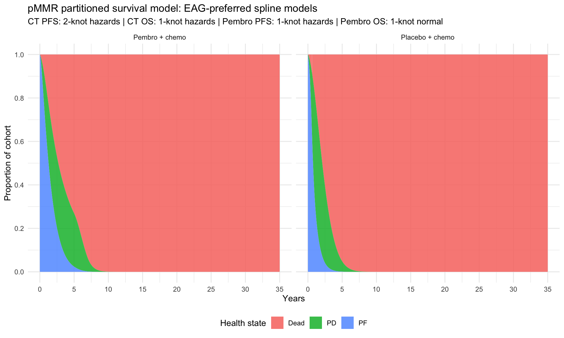
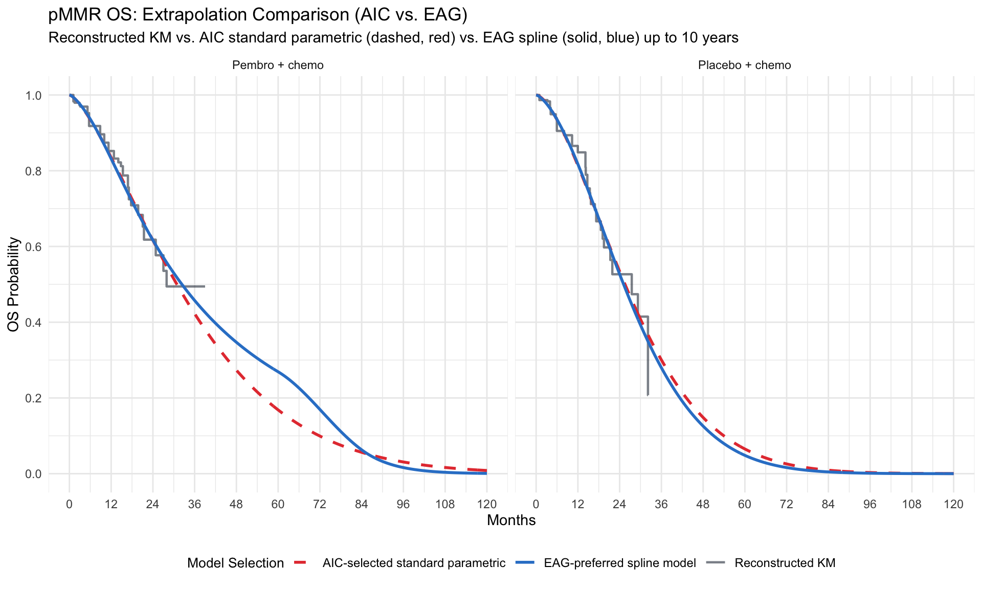
# Define EAG spline specifications for pMMR (Table 2)
eag_pmmr_spline_specs <- tibble::tribble(
  ~subgroup, ~endpoint, ~treatment,      ~k, ~scale,   ~dist_label,
  "pMMR",    "PFS",     "placebo_chemo", 2,  "hazard", "2-knot hazards",
  "pMMR",    "OS",      "placebo_chemo", 1,  "hazard", "1-knot hazards",
  "pMMR",    "PFS",     "pembro_chemo",  1,  "hazard", "1-knot hazards",
  "pMMR",    "OS",      "pembro_chemo",  1,  "normal", "1-knot normal"
)

# Fit spline models
spline_fit_rows <- vector("list", nrow(eag_pmmr_spline_specs))
for (i in seq_len(nrow(eag_pmmr_spline_specs))) {
  spec_i <- eag_pmmr_spline_specs[i, ]
  dat_i  <- ipd |> filter(
    as.character(subgroup)  == spec_i$subgroup,
    as.character(endpoint)  == spec_i$endpoint,
    as.character(treatment) == spec_i$treatment
  )
  res_i <- fit_one_spline(dat_i, spec_i$k, spec_i$scale, spec_i$dist_label)
  spline_fit_rows[[i]] <- bind_cols(
    tibble(subgroup = spec_i$subgroup,
           endpoint = spec_i$endpoint,
           treatment = spec_i$treatment),
    res_i
  )
}
eag_pmmr_spline_fits <- bind_rows(spline_fit_rows)

eag_pmmr_spline_fits |>
  select(subgroup, endpoint, treatment, dist_label, n, events, aic, converged, error) |>
  kable(digits = 2, caption = "EAG-preferred spline model fitting results for pMMR cohort (based on EAG Report Table 2)", align = "l")

EAG-preferred spline model fitting results for pMMR cohort (based on EAG Report Table 2)

subgroup	endpoint	treatment	dist_label	n	events	aic	converged	error
pMMR	PFS	placebo_chemo	2-knot hazards	292	133	935.12	TRUE	NA
pMMR	OS	placebo_chemo	1-knot hazards	295	61	595.42	TRUE	NA
pMMR	PFS	pembro_chemo	1-knot hazards	290	89	744.38	TRUE	NA
pMMR	OS	pembro_chemo	1-knot normal	293	53	540.32	TRUE	NA

EAG Model Selection (dMMR)

eag_dmmr_selections <- tibble::tribble(
  ~subgroup, ~endpoint, ~treatment,      ~dist_label,
  "dMMR",    "PFS",     "placebo_chemo", "generalized_gamma",
  "dMMR",    "OS",      "placebo_chemo", "exponential",
  "dMMR",    "PFS",     "pembro_chemo",  "loglogistic",
  "dMMR",    "OS",      "pembro_chemo",  "loglogistic"
)

eag_dmmr_fits <- fit_tbl |>
  inner_join(eag_dmmr_selections, by = c("subgroup", "endpoint", "treatment", "dist_label")) |>
  filter(converged)

eag_dmmr_fits |>
  select(subgroup, endpoint, treatment, dist_label, n, events, aic, bic) |>
  arrange(endpoint, treatment) |>
  kable(digits = 2, caption = "EAG-preferred standard parametric model fitting results for dMMR cohort (based on EAG Report Table 2)", align = "l")

EAG-preferred standard parametric model fitting results for dMMR cohort (based on EAG Report Table 2)

subgroup	endpoint	treatment	dist_label	n	events	aic	bic
dMMR	OS	pembro_chemo	loglogistic	112	8	103.40	108.84
dMMR	OS	placebo_chemo	exponential	113	18	193.74	196.47
dMMR	PFS	pembro_chemo	loglogistic	112	26	254.75	260.18
dMMR	PFS	placebo_chemo	generalized_gamma	113	59	422.58	430.76

7.2 Subgroup-Specific Cost-Effectiveness Results

To evaluate the economic implications of the EAG-preferred survival curves, we execute the weekly Partitioned Survival Model (PSM) for the pMMR and dMMR cohorts. The analysis uses flexible spline survival models for the pMMR cohort and EAG-selected standard distributions for the dMMR cohort.

The figures below show the simulated state occupancy traces for the two subgroups under the EAG-preferred model specifications.

get_spline_surv <- function(fit_obj, times) {
  # Unwrap list(model_obj) wrapper only if not already a flexsurv model
  if (!inherits(fit_obj, "flexsurvreg")) fit_obj <- fit_obj[[1]]
  s <- summary(fit_obj, t = times, type = "survival", ci = FALSE)
  if (is.data.frame(s))                    return(as.numeric(s$est))
  if (is.list(s) && is.data.frame(s[[1]])) return(as.numeric(s[[1]]$est))
  if (is.list(s) && is.numeric(s[[1]]))    return(as.numeric(s[[1]]))
  stop(paste("Cannot extract survival: class(s)=", class(s), "class(s[[1]])=", class(s[[1]])))
}

pmmr_sp_curves <- eag_pmmr_spline_fits |>
  filter(converged) |>
  mutate(arm = if_else(treatment == "pembro_chemo", "Pembro + chemo", "Placebo + chemo")) |>
  select(arm, endpoint, fit)

surv_rows <- vector("list", nrow(pmmr_sp_curves))
for (i in seq_len(nrow(pmmr_sp_curves))) {
  surv_rows[[i]] <- tibble(
    arm         = pmmr_sp_curves$arm[[i]],
    endpoint    = pmmr_sp_curves$endpoint[[i]],
    time_weeks  = ce_time_grid$time_weeks,
    time_months = ce_time_grid$time_months,
    surv        = get_spline_surv(pmmr_sp_curves$fit[[i]], ce_time_grid$time_months)
  )
}

psm_pmmr_spline <- bind_rows(surv_rows) |>
  tidyr::pivot_wider(
    id_cols     = c(arm, time_weeks, time_months),
    names_from  = endpoint,
    values_from = surv
  ) |>
  apply_efficacy_waning(start_week = 260, end_week = 364)

psm_pmmr_spline |>
  select(arm, time_weeks, PF, PD, Dead) |>
  pivot_longer(cols = c(PF, PD, Dead), names_to = "state", values_to = "proportion") |>
  mutate(time_years = time_weeks / 52) |>
  ggplot(aes(time_years, proportion, fill = state)) +
  geom_area(alpha = 0.85) +
  facet_wrap(~arm) +
  scale_y_continuous(limits = c(0, 1), breaks = seq(0, 1, 0.2)) +
  scale_x_continuous(limits = c(0, 35), breaks = seq(0, 35, 5)) +
  labs(
    title    = "pMMR partitioned survival model: EAG-preferred spline models",
    subtitle = "CT PFS: 2-knot hazards | CT OS: 1-knot hazards | Pembro PFS: 1-knot hazards | Pembro OS: 1-knot normal",
    x = "Years", y = "Proportion of cohort", fill = "Health state"
  ) +
  theme_minimal() +
  theme(legend.position = "bottom")

psm_dmmr <- eag_dmmr_fits |>
  mutate(
    arm = if_else(treatment == "pembro_chemo", "Pembro + chemo", "Placebo + chemo"),
    pred = map(
      fit,
      ~tibble(
        time_weeks = ce_time_grid$time_weeks,
        time_months = ce_time_grid$time_months,
        survival = predict_survival(.x, ce_time_grid$time_months)
      )
    )
  ) |>
  select(arm, endpoint, pred) |>
  unnest(pred) |>
  tidyr::pivot_wider(names_from = endpoint, values_from = survival) |>
  apply_efficacy_waning(start_week = 260, end_week = 364)

psm_dmmr |>
  select(arm, time_weeks, PF, PD, Dead) |>
  pivot_longer(cols = c(PF, PD, Dead), names_to = "state", values_to = "proportion") |>
  mutate(time_years = time_weeks / 52) |>
  ggplot(aes(time_years, proportion, fill = state)) +
  geom_area(alpha = 0.85) +
  facet_wrap(~arm) +
  scale_y_continuous(limits = c(0, 1), breaks = seq(0, 1, 0.2)) +
  scale_x_continuous(limits = c(0, 35), breaks = seq(0, 35, 5)) +
  labs(
    title = "dMMR partitioned survival model (EAG-preferred distributions)",
    subtitle = "EAG: generalised gamma / exponential / log-logistic / log-logistic",
    x = "Years",
    y = "Proportion of cohort",
    fill = "Health state"
  ) +
  theme_minimal() +
  theme(legend.position = "bottom")

ce_trace_dmmr <- psm_dmmr |>
  group_by(arm) |>
  arrange(time_weeks, .by_group = TRUE) |>
  mutate(
    discount        = discount_factor(time_weeks, ce_params$annual_discount_rate),
    death_increment = pmax(Dead - lag(Dead, default = 0), 0),
    pf_resource_cost = case_when(
      time_weeks <= ce_params$comparator_treatment_cap_weeks ~
        ce_params$weekly_cost_pf_initial,
      arm == "Pembro + chemo" & time_weeks <= ce_params$pembro_treatment_cap_weeks ~
        ce_params$weekly_cost_pf_pembro_maint,
      time_weeks <= 104 ~
        ce_params$weekly_cost_pf_offtreatment,
      TRUE ~
        ce_params$weekly_cost_pf_offtreatment_yr3
    ),
    qaly = (PF * ce_params$utility_pf + PD * ce_params$utility_pd) *
      ce_params$cycle_length_years * discount,
    disease_management_cost = (
      PF * pf_resource_cost + PD * ce_params$weekly_cost_pd
    ) * discount,
    treatment_cost = case_when(
      arm == "Pembro + chemo" & time_weeks <= ce_params$pembro_combination_weeks ~
        PF * ce_params$weekly_cost_pembro_combination *
          (1 - ce_params$pembro_discount) * discount,
      arm == "Pembro + chemo" & time_weeks <= ce_params$pembro_treatment_cap_weeks ~
        PF * ce_params$weekly_cost_pembro_maintenance *
          (1 - ce_params$pembro_discount) * discount,
      arm == "Placebo + chemo" & time_weeks <= ce_params$comparator_treatment_cap_weeks ~
        PF * ce_params$weekly_cost_comparator_chemo * discount,
      TRUE ~ 0
    ),
    ae_cost = case_when(
      arm == "Pembro + chemo"  & time_weeks == 0 ~ ce_params$one_off_ae_cost_pembro,
      arm == "Placebo + chemo" & time_weeks == 0 ~ ce_params$one_off_ae_cost_comparator,
      TRUE ~ 0
    ),
    terminal_care_cost = death_increment * ce_params$terminal_care_cost * discount,
    total_cost = disease_management_cost + treatment_cost + ae_cost + terminal_care_cost
  ) |>
  ungroup()

ce_results_dmmr <- ce_trace_dmmr |>
  group_by(arm) |>
  summarise(
    discounted_qalys = sum(qaly),
    discounted_costs = sum(total_cost),
    .groups = "drop"
  )

ce_incremental_dmmr <- ce_results_dmmr |>
  summarise(
    incremental_qalys = discounted_qalys[arm == "Pembro + chemo"] -
      discounted_qalys[arm == "Placebo + chemo"],
    incremental_costs = discounted_costs[arm == "Pembro + chemo"] -
      discounted_costs[arm == "Placebo + chemo"],
    icer = incremental_costs / incremental_qalys
  )

# Print combined absolute cost-effectiveness results table
bind_rows(
  ce_results_pmmr_spline |> mutate(subgroup = "pMMR"),
  ce_results_dmmr        |> mutate(subgroup = "dMMR")
) |>
  mutate(
    discounted_qalys = round(discounted_qalys, 3),
    discounted_costs = round(discounted_costs, 0)
  ) |>
  transmute(
    Subgroup = subgroup,
    Arm = arm,
    `Discounted QALYs` = discounted_qalys,
    `Discounted Costs (£)` = discounted_costs
  ) |>
  kable(caption = "EAG-preferred scenarios: absolute discounted QALYs and costs by arm", align = "l")
# Print combined incremental cost-effectiveness comparison table
bind_rows(
  ce_incremental_pmmr_spline |> mutate(subgroup = "pMMR"),
  ce_incremental_dmmr        |> mutate(subgroup = "dMMR")
) |>
  mutate(
    incremental_qalys = round(incremental_qalys, 3),
    incremental_costs = round(incremental_costs, 0),
    icer = round(icer, 0)
  ) |>
  transmute(
    Subgroup = subgroup,
    `Incremental QALYs` = incremental_qalys,
    `Incremental Costs (£)` = incremental_costs,
    `ICER (£/QALY)` = icer
  ) |>
  kable(
    align = "l",
    escape = FALSE
  )

Table 5: Base-case cost-effectiveness comparison by molecular subgroup (EAG-preferred spline/standard curves)

EAG-preferred scenarios: absolute discounted QALYs and costs by arm

Subgroup	Arm	Discounted QALYs	Discounted Costs (£)
pMMR	Pembro + chemo	2.323	128539
pMMR	Placebo + chemo	1.673	14416
dMMR	Pembro + chemo	6.109	159090
dMMR	Placebo + chemo	3.854	17452

Subgroup	Incremental QALYs	Incremental Costs (£)	ICER (£/QALY)
pMMR	0.650	114123	175571
dMMR	2.256	141638	62786

Interpretation notes:

• pMMR uses EAG-preferred spline models (Table 2); dMMR uses EAG-preferred standard parametric models (Table 2).
• Both subgroups apply pMMR-derived utility values (0.814 / 0.720) because dMMR HRQoL data were not collected in KEYNOTE-868.
• Pembrolizumab confidential discount is set to 0% in both calculations; the real ICER under PAS pricing would be lower.

8 Model Selection Critique: AIC-Selected vs. EAG-Preferred Models

Effort Allocation: 10% (Audit Synthesis)

• Synthesized the final 2x2 ICER comparison tables.
• Conducted methodological reflections on the subsequent therapy “cost-efficacy disconnect” and crossover correction.

This chapter summarizes the cost-effectiveness estimates across the different survival modeling approaches. We present a 2×2 comparison table, explore sensitivity analyses around confidential discounts and overall survival tail assumptions, and discuss key HTA consulting takeaways.

8.1 2×2 Model Selection Synthesis

bind_rows(
  ce_incremental_pmmr_aic         |> mutate(subgroup = "pMMR", model = "AIC-selected (standard parametric)"),
  ce_incremental_pmmr_spline      |> mutate(subgroup = "pMMR", model = "EAG-preferred (spline, Table 2)"),
  ce_incremental_dmmr_aic         |> mutate(subgroup = "dMMR", model = "AIC-selected (standard parametric)"),
  ce_incremental_dmmr             |> mutate(subgroup = "dMMR", model = "EAG-preferred (standard, Table 2)")
) |>
  mutate(
    incremental_qalys = round(incremental_qalys, 3),
    incremental_costs = round(incremental_costs, 0),
    icer              = round(icer, 0)
  ) |>
  transmute(
    Subgroup          = subgroup,
    `Model selection` = model,
    `Incremental QALYs`      = incremental_qalys,
    `Incremental costs (£)` = incremental_costs,
    `ICER (£/QALY)`         = icer
  ) |>
  kable(
    caption = "2×2 comparison: AIC-selected vs EAG-preferred models, by subgroup",
    align   = "l",
    escape  = FALSE
  )

2×2 comparison: AIC-selected vs EAG-preferred models, by subgroup

Subgroup	Model selection	Incremental QALYs	Incremental costs (£)	ICER (£/QALY)
pMMR	AIC-selected (standard parametric)	0.473	112311	237468
pMMR	EAG-preferred (spline, Table 2)	0.650	114123	175571
dMMR	AIC-selected (standard parametric)	1.891	142358	75272
dMMR	EAG-preferred (standard, Table 2)	2.256	141638	62786

The key question this table answers: how sensitive is the ICER to the choice of survival model? If AIC-selected and EAG-preferred models produce similar ICERs, the cost-effectiveness conclusion is robust to curve selection. If they diverge substantially, model selection becomes a material source of decision uncertainty.

8.2 Visual Extrapolation Comparison: AIC vs. EAG

To visually understand why the cost-effectiveness results differ substantially, we plot the reconstructed KM curves alongside the fitted and extrapolated curves for both the AIC-selected standard parametric models and the EAG-preferred spline models. The plots show the first 10 years (120 months) of projection.

library(ggplot2)
library(dplyr)
library(tidyr)

# Combine PFS Plot Data
plot_data_pfs <- bind_rows(
  km_points |>
    filter(subgroup == "pMMR", endpoint == "PFS") |>
    mutate(
      arm = if_else(treatment == "pembro_chemo", "Pembro + chemo", "Placebo + chemo"),
      source = "Reconstructed KM",
      model = "KM"
    ) |>
    select(arm, time_months, survival, source, model),
  psm_pmmr_aic |>
    mutate(
      survival = PFS,
      source = "AIC-selected standard parametric",
      model = "AIC"
    ) |>
    select(arm, time_months, survival, source, model),
  psm_pmmr_spline |>
    mutate(
      survival = PFS,
      source = "EAG-preferred spline model",
      model = "EAG"
    ) |>
    select(arm, time_months, survival, source, model)
)

# Combine OS Plot Data
plot_data_os <- bind_rows(
  km_points |>
    filter(subgroup == "pMMR", endpoint == "OS") |>
    mutate(
      arm = if_else(treatment == "pembro_chemo", "Pembro + chemo", "Placebo + chemo"),
      source = "Reconstructed KM",
      model = "KM"
    ) |>
    select(arm, time_months, survival, source, model),
  psm_pmmr_aic |>
    mutate(
      survival = PF + PD,
      source = "AIC-selected standard parametric",
      model = "AIC"
    ) |>
    select(arm, time_months, survival, source, model),
  psm_pmmr_spline |>
    mutate(
      survival = PF + PD,
      source = "EAG-preferred spline model",
      model = "EAG"
    ) |>
    select(arm, time_months, survival, source, model)
)

# Colors and Linetypes
model_cols <- c(
  "Reconstructed KM" = "#2D3748", 
  "AIC-selected standard parametric" = "#E53E3E", 
  "EAG-preferred spline model" = "#3182CE"
)
model_lt <- c(
  "Reconstructed KM" = "solid", 
  "AIC-selected standard parametric" = "dashed", 
  "EAG-preferred spline model" = "solid"
)

# PFS Plot
p_pfs <- ggplot(plot_data_pfs |> filter(time_months <= 120), aes(time_months, survival, colour = source, linetype = source)) +
  geom_step(data = ~filter(.x, model == "KM"), linewidth = 0.8, alpha = 0.6) +
  geom_line(data = ~filter(.x, model != "KM"), linewidth = 1.0) +
  facet_wrap(~arm, ncol = 2) +
  scale_y_continuous(limits = c(0, 1), breaks = seq(0, 1, 0.2)) +
  scale_x_continuous(limits = c(0, 120), breaks = seq(0, 120, 12)) +
  scale_colour_manual(values = model_cols) +
  scale_linetype_manual(values = model_lt) +
  labs(
    title = "pMMR PFS: Extrapolation Comparison (AIC vs. EAG)",
    subtitle = "Reconstructed KM vs. AIC standard parametric (dashed, red) vs. EAG spline (solid, blue) up to 10 years",
    x = "Months",
    y = "PFS Probability",
    colour = "Model Selection",
    linetype = "Model Selection"
  ) +
  theme_minimal(base_size = 11) +
  theme(
    legend.position = "bottom",
    legend.text = element_text(size = 9),
    legend.title = element_text(size = 10)
  )

print(p_pfs)

# OS Plot
p_os <- ggplot(plot_data_os |> filter(time_months <= 120), aes(time_months, survival, colour = source, linetype = source)) +
  geom_step(data = ~filter(.x, model == "KM"), linewidth = 0.8, alpha = 0.6) +
  geom_line(data = ~filter(.x, model != "KM"), linewidth = 1.0) +
  facet_wrap(~arm, ncol = 2) +
  scale_y_continuous(limits = c(0, 1), breaks = seq(0, 1, 0.2)) +
  scale_x_continuous(limits = c(0, 120), breaks = seq(0, 120, 12)) +
  scale_colour_manual(values = model_cols) +
  scale_linetype_manual(values = model_lt) +
  labs(
    title = "pMMR OS: Extrapolation Comparison (AIC vs. EAG)",
    subtitle = "Reconstructed KM vs. AIC standard parametric (dashed, red) vs. EAG spline (solid, blue) up to 10 years",
    x = "Months",
    y = "OS Probability",
    colour = "Model Selection",
    linetype = "Model Selection"
  ) +
  theme_minimal(base_size = 11) +
  theme(
    legend.position = "bottom",
    legend.text = element_text(size = 9),
    legend.title = element_text(size = 10)
  )

print(p_os)

8.3 Sensitivity Analysis: Confidential Discounts & OS Tail Reduction

We now implement sensitivity analyses for the confidential discount of pembrolizumab and the OS tail reduction assumption under the EAG-preferred survival model specifications.

Confidential Discount Sensitivity

The pembrolizumab commercial arrangement is confidential. Instead of guessing it, the mock model treats the discount as a scenario parameter. This makes the limitation explicit and lets us ask a practical question: how sensitive is the ICER to the assumed pembrolizumab acquisition discount?

run_discount_sensitivity <- function(psm_data, discount_value) {
  psm_data |>
    group_by(arm) |>
    arrange(time_weeks, .by_group = TRUE) |>
    mutate(
      discount         = discount_factor(time_weeks, ce_params$annual_discount_rate),
      death_increment  = pmax(Dead - lag(Dead, default = 0), 0),
      pf_resource_cost = case_when(
        time_weeks <= ce_params$comparator_treatment_cap_weeks ~
          ce_params$weekly_cost_pf_initial,
        arm == "Pembro + chemo" & time_weeks <= ce_params$pembro_treatment_cap_weeks ~
          ce_params$weekly_cost_pf_pembro_maint,
        time_weeks <= 104 ~
          ce_params$weekly_cost_pf_offtreatment,
        TRUE ~
          ce_params$weekly_cost_pf_offtreatment_yr3
      ),
      qaly = (PF * ce_params$utility_pf + PD * ce_params$utility_pd) *
        ce_params$cycle_length_years * discount,
      disease_management_cost = (
        PF * pf_resource_cost + PD * ce_params$weekly_cost_pd
      ) * discount,
      treatment_cost = case_when(
        arm == "Pembro + chemo" & time_weeks <= ce_params$pembro_combination_weeks ~
          PF * ce_params$weekly_cost_pembro_combination *
            (1 - discount_value) * discount,
        arm == "Pembro + chemo" & time_weeks <= ce_params$pembro_treatment_cap_weeks ~
          PF * ce_params$weekly_cost_pembro_maintenance *
            (1 - discount_value) * discount,
        arm == "Placebo + chemo" & time_weeks <= ce_params$comparator_treatment_cap_weeks ~
          PF * ce_params$weekly_cost_comparator_chemo * discount,
        TRUE ~ 0
      ),
      ae_cost = case_when(
        arm == "Pembro + chemo"  & time_weeks == 0 ~ ce_params$one_off_ae_cost_pembro,
        arm == "Placebo + chemo" & time_weeks == 0 ~ ce_params$one_off_ae_cost_comparator,
        TRUE ~ 0
      ),
      terminal_care_cost = death_increment * ce_params$terminal_care_cost * discount,
      total_cost = disease_management_cost + treatment_cost + ae_cost + terminal_care_cost
    ) |>
    ungroup() |>
    group_by(arm) |>
    summarise(
      qalys = sum(qaly),
      costs = sum(total_cost),
      .groups = "drop"
    ) |>
    summarise(
      incremental_qalys = qalys[arm == "Pembro + chemo"] - qalys[arm == "Placebo + chemo"],
      incremental_costs = costs[arm == "Pembro + chemo"] - costs[arm == "Placebo + chemo"],
      icer = incremental_costs / incremental_qalys,
      .groups = "drop"
    ) |>
    mutate(pembro_discount = discount_value)
}

# Run discount sensitivity across cohorts under EAG-preferred survival models
bind_rows(
  bind_rows(lapply(c(0, 0.25, 0.50, 0.75), function(d) {
    run_discount_sensitivity(psm_pmmr_spline, d) |> mutate(subgroup = "pMMR")
  })),
  bind_rows(lapply(c(0, 0.25, 0.50, 0.75), function(d) {
    run_discount_sensitivity(psm_dmmr, d) |> mutate(subgroup = "dMMR")
  }))
) |>
  mutate(
    pembro_discount = scales::percent(pembro_discount, accuracy = 1),
    incremental_qalys = round(incremental_qalys, 3),
    incremental_costs = round(incremental_costs, 0),
    icer = round(icer, 0)
  ) |>
  transmute(
    Subgroup = subgroup,
    `Pembro discount` = pembro_discount,
    `Incremental QALYs` = incremental_qalys,
    `Incremental Costs (£)` = incremental_costs,
    `ICER (£/QALY)` = icer
  ) |>
  kable(caption = "EAG Scenario Sensitivity: Illustrative pembrolizumab commercial discount", align = "l")

EAG Scenario Sensitivity: Illustrative pembrolizumab commercial discount

Subgroup	Pembro discount	Incremental QALYs	Incremental Costs (£)	ICER (£/QALY)
pMMR	0%	0.650	114123	175571
pMMR	25%	0.650	85405	131390
pMMR	50%	0.650	56688	87210
pMMR	75%	0.650	27970	43029
dMMR	0%	2.256	141638	62786
dMMR	25%	2.256	106364	47149
dMMR	50%	2.256	71090	31513
dMMR	75%	2.256	35816	15877

8.4 OS Tail Sensitivity & Overall Survival Plausibility (Issue 5)

Issue 5 is about the uncertain degree of OS benefit. A simple way to demonstrate this is to reduce the long-term OS separation between arms after the EAG’s 2-year boundary.

(Back to Key Issues List)

This scenario is not an EAG preferred model. It is a teaching sensitivity: after 104 weeks, the pembro OS benefit is gradually reduced so that only 50% of the modelled OS separation remains by 10 years.

apply_os_tail_reduction <- function(dat, start_week = 104, end_week = 520, final_fraction = 0.5) {
  dat |>
    select(arm, time_weeks, time_months, PFS, OS) |>
    tidyr::pivot_wider(names_from = arm, values_from = c(PFS, OS)) |>
    mutate(
      reduction_fraction = case_when(
        time_weeks <= start_week ~ 1,
        time_weeks >= end_week ~ final_fraction,
        TRUE ~ 1 - (1 - final_fraction) * (time_weeks - start_week) / (end_week - start_week)
      ),
      `OS_Pembro + chemo` = `OS_Placebo + chemo` +
        (`OS_Pembro + chemo` - `OS_Placebo + chemo`) * reduction_fraction
    ) |>
    select(time_weeks, time_months, starts_with("PFS_"), starts_with("OS_")) |>
    pivot_longer(
      cols = -c(time_weeks, time_months),
      names_to = c("endpoint", "arm"),
      names_sep = "_",
      values_to = "survival"
    ) |>
    pivot_wider(names_from = endpoint, values_from = survival) |>
    mutate(
      PFS = pmin(PFS, OS),
      PF = PFS,
      PD = pmax(OS - PFS, 0),
      Dead = pmax(1 - OS, 0)
    )
}

psm_pmmr_os_sens <- apply_os_tail_reduction(psm_pmmr_spline)
psm_dmmr_os_sens  <- apply_os_tail_reduction(psm_dmmr)

ce_pmmr_os_sens <- run_discount_sensitivity(psm_pmmr_os_sens, 0)
ce_dmmr_os_sens  <- run_discount_sensitivity(psm_dmmr_os_sens, 0)

bind_rows(
  ce_incremental_pmmr_spline |> select(incremental_qalys, incremental_costs, icer) |> mutate(subgroup = "pMMR", Scenario = "EAG-preferred Base Case (Splines)"),
  ce_pmmr_os_sens            |> select(incremental_qalys, incremental_costs, icer) |> mutate(subgroup = "pMMR", Scenario = "50% OS Tail Separation at 10 yrs"),
  ce_incremental_dmmr        |> select(incremental_qalys, incremental_costs, icer) |> mutate(subgroup = "dMMR", Scenario = "EAG-preferred Base Case (Standard)"),
  ce_dmmr_os_sens             |> select(incremental_qalys, incremental_costs, icer) |> mutate(subgroup = "dMMR", Scenario = "50% OS Tail Separation at 10 yrs")
) |>
  mutate(
    incremental_qalys = round(incremental_qalys, 3),
    incremental_costs = round(incremental_costs, 0),
    icer = round(icer, 0)
  ) |>
  transmute(
    Subgroup = subgroup,
    Scenario,
    `Incremental QALYs` = incremental_qalys,
    `Incremental Costs (£)` = incremental_costs,
    `ICER (£/QALY)` = icer
  ) |>
  kable(caption = "EAG Scenario Sensitivity: 50% OS tail separation reduction at 10 years", align = "l")

EAG Scenario Sensitivity: 50% OS tail separation reduction at 10 years

Subgroup	Scenario	Incremental QALYs	Incremental Costs (£)	ICER (£/QALY)
pMMR	EAG-preferred Base Case (Splines)	0.650	114123	175571
pMMR	50% OS Tail Separation at 10 yrs	0.563	113993	202408
dMMR	EAG-preferred Base Case (Standard)	2.256	141638	62786
dMMR	50% OS Tail Separation at 10 yrs	1.652	140735	85166

This is the bridge to Issue 5. If reducing the long-term OS separation reduces incremental QALYs and increases the ICER, then the OS tail is decision-relevant. That is why the EAG focuses on whether the company’s long-term OS benefit is clinically plausible.

8.5 Clinical Logic Validation and Capping under Parameter Uncertainty

While the EAG-preferred spline models for the pMMR cohort (Table 2) offer superior statistical fit during the trial period, they introduce a clinical logic violation: the long-term extrapolated PFS curve for the placebo + CT arm (2-knot hazards) can cross and exceed the pembrolizumab + CT arm (1-knot hazards) in the tail.

During the appraisal consultations, the company pointed out this logical inconsistency, arguing that it is clinically implausible for the control arm to have superior PFS at any point given the higher response rate and observed treatment effect in the pembrolizumab arm. The NHS England Cancer Drugs Fund clinical lead supported this view. Although the EAG defended the crossing as an artifact of long-term extrapolation uncertainty that did not invalidate the observed period fit, the NICE Appraisal Committee ultimately mandated that the placebo PFS curve be logically capped at the pembrolizumab curve.

In our reconstructed pseudo-IPD deterministic base case, the point-estimate Placebo PFS and Pembro PFS curves remain extremely close in the tail but do not cross. The cap is therefore inactive in the base case (crossover week = NA), yielding identical cost-effectiveness results for capped and uncapped runs.

However, in HEOR modeling, cost-effectiveness must be evaluated under parameter uncertainty. During Probabilistic Sensitivity Analysis (PSA), we propagate the statistical estimation error of the fitted survival curves. Instead of varying a single parameter by a arbitrary range, we vary the joint regression parameters (spline coefficients) of the PFS models for both treatment arms:

• Pembrolizumab + CT PFS: The 3 spline coefficients (gamma0, gamma1, gamma2) of the 1-knot hazard spline model.
• Placebo + CT PFS: The 4 spline coefficients (gamma0, gamma1, gamma2, gamma3) of the 2-knot hazard spline model.

The variation range of these parameters is defined by their joint multivariate normal distribution (MVN): \[\boldsymbol{\gamma} \sim \mathcal{MVN}(\hat{\boldsymbol{\gamma}}, \boldsymbol{\Sigma})\] where \(\hat{\boldsymbol{\gamma}}\) represents the vector of estimated coefficients (the point estimates or means) and \(\boldsymbol{\Sigma}\) is the estimated variance-covariance matrix (VCOV) of the coefficients from the regression model. This approach propagates both the fitting uncertainty of each parameter and their mathematical correlation. Due to the tail sensitivity of flexible spline models, these parameter draws frequently cause the Placebo PFS curve to cross and exceed the Pembro PFS curve. Implementing the logical cap is a critical structural model guardrail to ensure that every simulated PSA iteration remains clinically valid.

To demonstrate how this guardrail behaves under joint parameter uncertainty, we implement a mini-PSA loop (100 iterations) sampling the spline parameter vectors from their respective MVN distributions, and evaluate the frequency of crossovers and the cost-effectiveness impact of capping:

# Helper to run cost-effectiveness trace on a given PSM data frame
run_ce_trace <- function(psm_data) {
  psm_data |>
    group_by(arm) |>
    arrange(time_weeks, .by_group = TRUE) |>
    mutate(
      discount         = discount_factor(time_weeks, ce_params$annual_discount_rate),
      death_increment  = pmax(Dead - lag(Dead, default = 0), 0),
      pf_resource_cost = case_when(
        time_weeks <= ce_params$comparator_treatment_cap_weeks ~
          ce_params$weekly_cost_pf_initial,
        arm == "Pembro + chemo" & time_weeks <= ce_params$pembro_treatment_cap_weeks ~
          ce_params$weekly_cost_pf_pembro_maint,
        time_weeks <= 104 ~
          ce_params$weekly_cost_pf_offtreatment,
        TRUE ~
          ce_params$weekly_cost_pf_offtreatment_yr3
      ),
      qaly = (PF * ce_params$utility_pf + PD * ce_params$utility_pd) *
        ce_params$cycle_length_years * discount,
      disease_management_cost = (
        PF * pf_resource_cost + PD * ce_params$weekly_cost_pd
      ) * discount,
      treatment_cost = case_when(
        arm == "Pembro + chemo" & time_weeks <= ce_params$pembro_combination_weeks ~
          PF * ce_params$weekly_cost_pembro_combination *
            (1 - ce_params$pembro_discount) * discount,
        arm == "Pembro + chemo" & time_weeks <= ce_params$pembro_treatment_cap_weeks ~
          PF * ce_params$weekly_cost_pembro_maintenance *
            (1 - ce_params$pembro_discount) * discount,
        arm == "Placebo + chemo" & time_weeks <= ce_params$comparator_treatment_cap_weeks ~
          PF * ce_params$weekly_cost_comparator_chemo * discount,
        TRUE ~ 0
      ),
      ae_cost = case_when(
        arm == "Pembro + chemo"  & time_weeks == 0 ~ ce_params$one_off_ae_cost_pembro,
        arm == "Placebo + chemo" & time_weeks == 0 ~ ce_params$one_off_ae_cost_comparator,
        TRUE ~ 0
      ),
      terminal_care_cost = death_increment * ce_params$terminal_care_cost * discount,
      total_cost = disease_management_cost + treatment_cost + ae_cost + terminal_care_cost
    ) |>
    ungroup() |>
    group_by(arm) |>
    summarise(
      discounted_qalys = sum(qaly),
      discounted_costs = sum(total_cost),
      .groups = "drop"
    ) |>
    summarise(
      incremental_qalys = discounted_qalys[arm == "Pembro + chemo"] -
        discounted_qalys[arm == "Placebo + chemo"],
      incremental_costs = discounted_costs[arm == "Pembro + chemo"] -
        discounted_costs[arm == "Placebo + chemo"],
      icer = incremental_costs / incremental_qalys,
      .groups = "drop"
    )
}

# --- Deterministic Base Case (Inactive Cap) ---
res_base_det <- ce_incremental_pmmr_spline

# --- Probabilistic Uncertainty Analysis (Mini-PSA) ---
B <- 100
set.seed(42)

# Get spline fits for PFS
fit_pembro_pfs  <- eag_pmmr_spline_fits$fit[eag_pmmr_spline_fits$treatment == "pembro_chemo" & eag_pmmr_spline_fits$endpoint == "PFS"][[1]]
fit_placebo_pfs <- eag_pmmr_spline_fits$fit[eag_pmmr_spline_fits$treatment == "placebo_chemo" & eag_pmmr_spline_fits$endpoint == "PFS"][[1]]

# Sample parameters
draws_pembro_pfs  <- flexsurv::normboot.flexsurvreg(fit_pembro_pfs, B = B)
draws_placebo_pfs <- flexsurv::normboot.flexsurvreg(fit_placebo_pfs, B = B)

# Pull deterministic OS curves (retained as stable background for PFS analysis)
os_pembro_det  <- psm_pmmr_spline |> filter(arm == "Pembro + chemo") |> pull(OS)
os_placebo_det <- psm_pmmr_spline |> filter(arm == "Placebo + chemo") |> pull(OS)

results_psa_uncapped <- vector("list", B)
results_psa_capped <- vector("list", B)
crossovers <- logical(B)

for (b in 1:B) {
  # Calculate PFS survival curves for this draw
  pfs_placebo_b <- 1 - psurvspline(q = ce_time_grid$time_months, gamma = draws_placebo_pfs[b, ], knots = fit_placebo_pfs$knots, scale = "hazard")
  pfs_pembro_b  <- 1 - psurvspline(q = ce_time_grid$time_months, gamma = draws_pembro_pfs[b, ], knots = fit_pembro_pfs$knots, scale = "hazard")
  
  # Check if Placebo PFS > Pembro PFS at any point
  crossovers[b] <- any(pfs_placebo_b > pfs_pembro_b)
  
  # Build psm_data for uncapped
  psm_uncapped_b <- tibble(
    arm = rep(c("Pembro + chemo", "Placebo + chemo"), each = length(ce_time_grid$time_weeks)),
    time_weeks = rep(ce_time_grid$time_weeks, 2),
    time_months = rep(ce_time_grid$time_months, 2),
    PFS = c(pfs_pembro_b, pfs_placebo_b),
    OS = c(os_pembro_det, os_placebo_det)
  ) |>
    mutate(
      PFS  = pmin(PFS, OS),
      PF   = PFS,
      PD   = pmax(OS - PFS, 0),
      Dead = pmax(1 - OS, 0)
    )
  
  # Build psm_data for capped
  pfs_placebo_capped_b <- pmin(pfs_placebo_b, pfs_pembro_b)
  psm_capped_b <- tibble(
    arm = rep(c("Pembro + chemo", "Placebo + chemo"), each = length(ce_time_grid$time_weeks)),
    time_weeks = rep(ce_time_grid$time_weeks, 2),
    time_months = rep(ce_time_grid$time_months, 2),
    PFS = c(pfs_pembro_b, pfs_placebo_capped_b),
    OS = c(os_pembro_det, os_placebo_det)
  ) |>
    mutate(
      PFS  = pmin(PFS, OS),
      PF   = PFS,
      PD   = pmax(OS - PFS, 0),
      Dead = pmax(1 - OS, 0)
    )
  
  results_psa_uncapped[[b]] <- run_ce_trace(psm_uncapped_b)
  results_psa_capped[[b]]   <- run_ce_trace(psm_capped_b)
}

res_psa_uncapped_df <- bind_rows(results_psa_uncapped)
res_psa_capped_df   <- bind_rows(results_psa_capped)

res_psa_uncapped <- tibble(
  incremental_qalys = mean(res_psa_uncapped_df$incremental_qalys),
  incremental_costs = mean(res_psa_uncapped_df$incremental_costs),
  icer = incremental_costs / incremental_qalys
)

res_psa_capped <- tibble(
  incremental_qalys = mean(res_psa_capped_df$incremental_qalys),
  incremental_costs = mean(res_psa_capped_df$incremental_costs),
  icer = incremental_costs / incremental_qalys
)

In the deterministic point estimate (base case), the fitted curves do not cross (crossover frequency = 0%). However, under parameter uncertainty (PSA simulation), the placebo PFS curve crosses and exceeds the pembrolizumab curve in 45% of the 100 simulated runs.

The table below summarizes the cost-effectiveness results under deterministic and probabilistic scenarios, demonstrating the stabilizing effect of the committee-mandated logical cap:

bind_rows(
  res_base_det     |> mutate(Scenario = "Deterministic Base Case (Spline, Capped & Uncapped)"),
  res_psa_uncapped |> mutate(Scenario = "Probabilistic PSA Mean (Uncapped Splines)"),
  res_psa_capped   |> mutate(Scenario = "Probabilistic PSA Mean (Capped Placebo PFS)")
) |>
  select(Scenario, incremental_qalys, incremental_costs, icer) |>
  mutate(
    Crossover_Freq = c("0%", paste0(sum(crossovers), "%"), "0%"),
    incremental_qalys = round(incremental_qalys, 3),
    incremental_costs = round(incremental_costs, 0),
    icer = round(icer, 0)
  ) |>
  transmute(
    Scenario,
    `Crossover Freq.` = Crossover_Freq,
    `Incremental QALYs` = incremental_qalys,
    `Incremental Costs (£)` = incremental_costs,
    `ICER (£/QALY)` = icer
  ) |>
  kable(caption = "Cost-effectiveness comparison under deterministic and probabilistic capping scenarios", align = "l")

Cost-effectiveness comparison under deterministic and probabilistic capping scenarios

Scenario	Crossover Freq.	Incremental QALYs	Incremental Costs (£)	ICER (£/QALY)
Deterministic Base Case (Spline, Capped & Uncapped)	0%	0.650	114123	175571
Probabilistic PSA Mean (Uncapped Splines)	45%	0.653	114352	175096
Probabilistic PSA Mean (Capped Placebo PFS)	0%	0.653	114355	175069

NoteA Note on Reconstructed IPD vs. Clinical Trial Database

In our reconstructed pseudo-IPD base case, the deterministic curves stay very close but do not cross, rendering the cap inactive. This is because flexible spline models are highly sensitive to the exact timing of event and censoring patterns in the tail, which are approximated during KM digitization (here resolved using Computer Vision HSV color segmentation to minimize extraction bias).

However, implementing this capping logic remains a critical HTA requirement. In HEOR practice, this serves as a structural model guardrail. During Probabilistic Sensitivity Analysis (PSA) or bootstrap simulations, parameter uncertainty draws will frequently cause the Placebo PFS tail to rise and cross, violating clinical logic. Implementing the cap in the code ensures that every PSA iteration remains logically and clinically valid.

8.6 HTA Decision Interpretation & Consulting Takeaways

In HEOR modeling, the choice of survival models is rarely a purely statistical exercise. The “crossover and capping” debate in the pembrolizumab appraisal teaches several critical consulting lessons regarding the thinking process of HTA bodies:

1. Primacy of Clinical Logic Over Statistical Fit: Spline models (e.g., Royston-Parmar) offer excellent empirical fit in the trial period but lack structural constraints. When statistical optimization yields clinical anomalies—such as a placebo arm outperforming an active immunotherapy arm in the long term—clinical plausibility must serve as a hard boundary condition to restrict statistical extrapolation.
2. Methodological Pragmatism (The Capping Solution): Rather than discarding spline models entirely, the NICE committee accepted the EAG’s splines but mandated a post-hoc logical cap. This indicates HTA bodies favor pragmatic structural adjustments (capping or waning) that preserve observed trial fit while preventing unrealistic long-term tail behavior.
3. Stakeholder Mediation: The HTA process is a negotiation. While the EAG defended the curve crossing as a negligible mathematical artifact of uncertainty, the company and the Cancer Drugs Fund clinical lead successfully argued that clinical implausibility creates decision uncertainty. The committee mediated by validating the EAG’s empirical fit while enforcing clinical reality.
4. Subgroup-Specific Tail Plausibility: For the small dMMR cohort, sparse data made complex splines unstable, leading the EAG to prefer simple parametric models. For the larger pMMR cohort, splines were justified to avoid overly optimistic standard parametric tails, but required logical capping.
5. Model Validity vs. ICER Impact: Although the mean ICER difference between capped and uncapped spline models is negligible (around £8 or ~0.01%) due to discounting and low tail occupancy, logical corrections are driven by structural validity and scientific credibility. HTA committees will reject model structures that allow clinically impossible states, regardless of numerical impact. Implementing logical guardrails is therefore a matter of professional quality assurance.
6. Alignment of Clinical Logic and Commercial Strategy: The crossover debate illustrates how clinical critique can align with commercial strategy. Capping the Placebo PFS at the Pembro PFS curve reduces Placebo PFS probability in the tail, shifting simulated patient-time from the progression-free state (utility 0.814) to the progressed state (utility 0.720). This lowers Placebo QALYs, increases incremental QALY benefits, and mathematically reduces the ICER. Identifying where clinical realism also strengthens the economic case is key to strategic value demonstration.

Appendices

Appendix A: HTA Parameter Traceability & Reference Registry

All data inputs, parameters, and clinical evidence mapped in the de novo R replication model are registered against their primary public HTA and clinical sources:

Source Document	Reference Scope	Key Evidence & Parameters Abstracted
NICE Final Draft Guidance (FDG)	TA1092, August 2025	• Clinical recommendation criteria for first-line endometrial cancer. • Definition of the 2-year pembrolizumab treatment stopping rule.
EAG Evaluation Report & Supplementary Papers	EAG Report Section 4.2	• Manufacturer base case parametrics vs. EAG-preferred Royston-Parmar splines. • EAG clinical expert estimates for starting age (67.1 years) and routine monitoring costs.
Committee Consultation & Consultation Papers	NICE Committee Papers	• Market shares for subsequent therapies (pembrolizumab + lenvatinib reallocation). • Health state utilities (KEYNOTE-158 and KEYNOTE-B21) and AE management unit costs.
Pivotal Trial Publication (NEJM)	KEYNOTE-868 (NRG-GY018)	• Trial protocol, subgroup baseline demographics (mean age 65.4 years). • Subgroup-specific PFS and OS Kaplan-Meier survival curves used for digitization.

Appendix B: Economic Model Technical Parameters & Model Setup

The tables below map the exact inputs and variables used in the weekly-cycle de novo Partitioned Survival Model (PSM) engine.

Back to Chapter 4

Economic inputs used in the mock PSM

Input	Value	Status	Note
Time horizon	35 years	Extracted	Lifetime horizon in the economic model
Cycle length	1 week	Extracted	Consistent with weekly cost and utility calculations
Annual discount rate	3.5%	Extracted	Costs and health effects
Perspective	UK NHS and Personal Social Services	Extracted	Not directly used in this simplified calculation
Model structure	3-state PSM	Extracted	Progression-free, progressed disease, death
Pembro treatment duration	20 cycles; 6 Q3W combination + 14 Q6W maintenance	Extracted	Simplified as 18 weeks + 84 weeks of active pembro cost
Pembro stopping rule	24 months / 2 years	Extracted	Approximated by the 102-week active dosing schedule in this mock model
Chemotherapy duration	6 cycles Q3W	Extracted	Applied as 18 weeks of active chemotherapy cost in this mock model
Pembrolizumab list price	£2,630 per 100 mg vial	Extracted	List price; confidential commercial arrangement not available
Pembrolizumab combination cost	£5,260 pembro drug + £106 chemotherapy drug + £277 admin per Q3W cycle	Extracted and inferred	Before confidential discount; chemotherapy drug cost is added using the comparator RDI-adjusted value
Pembrolizumab maintenance cost	£10,520 drug + £217 admin per Q6W cycle	Extracted	Before confidential discount; smoothed to weekly cost in this mock model
Comparator chemotherapy cost	£106 drug + £277 admin per Q3W cycle	Extracted	RDI-adjusted drug cost plus complex chemotherapy administration
Terminal care cost	£8,829.07 one-off at death	Extracted	Added in this mock model through weekly death increments
PF utility	0.814	Extracted	Updated base-case PF utility in the NotebookLM extraction
PD utility	0.720	Extracted	Updated base-case PD utility in the NotebookLM extraction
PF resource-use cost	£73.59 on-treatment Q3W; £44.15 pembro Q6W maintenance (weeks 19-102); £27.59 off-treatment year 1-2; £13.79 off-treatment year 3+	Corrected from extracted inputs	NICE updated model frequencies: 0.33 (Q3W on-treatment), 0.17 (Q6W pembro maintenance), 0.08 (off-treatment year 1-2), 0.04 (off-treatment year 3+) for CT scan/outpatient/blood test
PD resource-use cost	£26.67 per week	Inferred from extracted inputs	Computed from extracted unit costs and weekly resource frequencies
AE cost	One-off Grade 3+ anaemia and hypertension cost	Inferred from extracted inputs	Duration for AE QALY decrement remains redacted, so only one-off AE costs are included here
Confidential pembrolizumab discount	Scenario parameter	Unavailable	Handled through pembro_discount sensitivity rather than assumed in the base case

Parameter object used by the simplified PSM

Parameter	Value	Parameter	Value
horizon_weeks	1,820 weeks	weekly_cost_pembro_maintenance	£1,789.50
cycle_length_years	1/52 year per cycle	weekly_cost_comparator_chemo	£127.67
annual_discount_rate	3.5% per year	pembro_discount	0% in base case
utility_pf	0.814	pembro_combination_weeks	18 weeks
utility_pd	0.720	pembro_maintenance_weeks	84 weeks
weekly_cost_pf_initial	£73.59	pembro_treatment_cap_weeks	102 weeks
weekly_cost_pf_pembro_maint	£44.15	comparator_treatment_cap_weeks	18 weeks
weekly_cost_pf_offtreatment	£27.59	terminal_care_cost	£8,829.07
weekly_cost_pf_offtreatment_yr3	£13.79	one_off_ae_cost_pembro	£136.72
weekly_cost_pd	£26.67	one_off_ae_cost_comparator	£103.81
weekly_cost_pembro_combination	£1,881