Mock Case — Survival Extrapolation in a Partitioned Survival Model

Treatment Effect Waning and Recursive Hazard Chaining: Isavetinib in Relapsed/Refractory Multiple Myeloma

Author

Xiaoge Zhang, PhD

Published

June 1, 2026

Mock Case Disclosure

This is a methodological demonstration using fully synthetic parameters. The clinical scenario — Isavetinib versus standard of care (SoC) in Relapsed/Refractory Multiple Myeloma (RRMM) — is fictional and designed to expose a real methodological challenge in oncology HTA submissions: how to model treatment effect waning beyond the trial observation window in a biologically defensible way.

1 Executive Summary

Standard oncology HTA submissions in England require a 30-year (lifetime) model horizon, yet pivotal trials for RRMM typically provide 3–5 years of follow-up data. This creates the extrapolation problem: how should the treatment benefit observed during the trial period be projected forward?

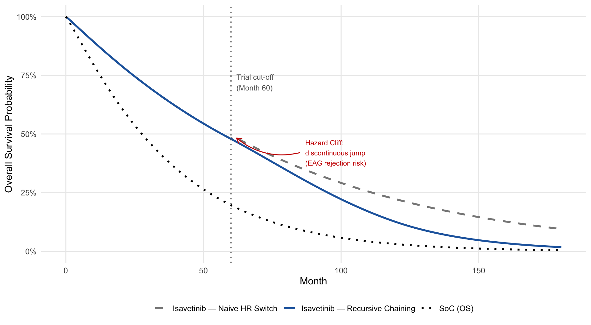
A common, computationally simple approach is to apply a constant Hazard Ratio (HR) at the trial cut-off point. This case demonstrates that this approach generates a mathematically discontinuous “Hazard Cliff” at the extrapolation boundary — a structural artefact that NICE Evidence Assessment Groups (EAGs) routinely flag as biologically implausible.

This case study develops and validates an alternative: Recursive Hazard Chaining, which anchors the long-term extrapolation to the trial-period hazard at the cut-off point and applies a clinically motivated linear waning function. The result is a smooth, continuous survival trajectory that is far more defensible in front of an appraisal committee.

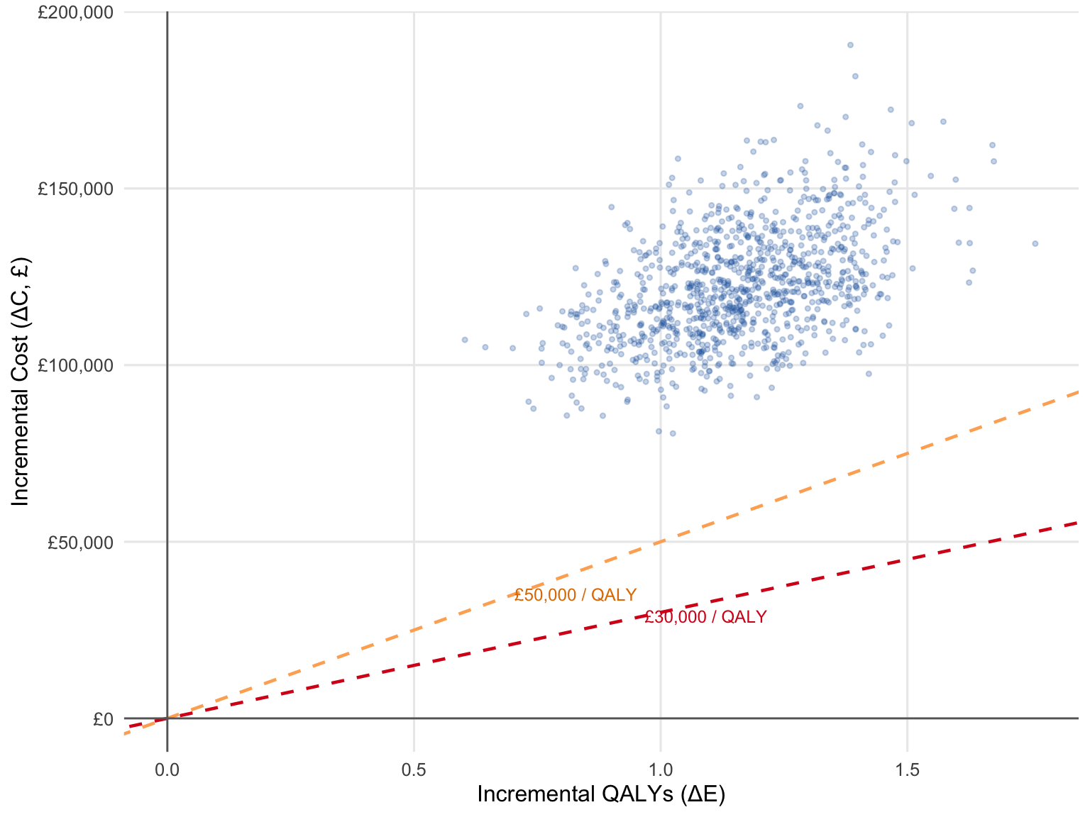
Base-case results: ICER = £53,514 / QALY (\(\Delta C\): £34,761 | \(\Delta E\): 0.649 QALYs). The full probabilistic sensitivity analysis (1,000 iterations) yields a 51% probability of cost-effectiveness at the £50,000 severity-adjusted threshold.

2 Decision Problem & Clinical Background

Multiple myeloma is a haematological malignancy of plasma cells with a median age at diagnosis of approximately 70 years. Virtually all patients eventually relapse, and each successive line of therapy is associated with shorter remission and reduced performance status. In the RRMM setting, the key clinical endpoint is Progression-Free Survival (PFS), with Overall Survival (OS) as the co-primary or secondary endpoint.

Isavetinib (fictional) is a novel oral kinase inhibitor being evaluated against a SoC backbone in the third-line RRMM setting. A company-sponsored trial provided 60 months of individual patient follow-up. The modelled base-case parameters are calibrated to reflect a realistic RRMM scenario:

SoC median OS: ~24 months
Isavetinib median OS: ~50 months (HR ≈ 0.55)
Model horizon: 30 years (360 monthly cycles)

The central methodological challenge is that the treatment benefit observed at Month 60 cannot plausibly be assumed to persist unchanged at its trial-period magnitude into Years 10, 20, and 30.

3 The Partitioned Survival Model: Mathematical Framework

3.1 Three-State Structure

A Partitioned Survival Model (PSM) is defined by two independent survival functions — PFS and OS — that jointly determine the proportion of the cohort in each of three mutually exclusive health states at every model cycle.

Notation. Let \(S_{\text{PFS}}(t)\) and \(S_{\text{OS}}(t)\) denote the survival functions for progression-free survival and overall survival respectively, where \(S(t) \in [0,1]\) is the probability of not having experienced the corresponding event by time \(t\). Let \(\pi_k(t)\) denote the state occupancy probability for health state \(k\) at time \(t\) — the proportion of the cohort residing in state \(k\) at cycle \(t\). The key structural feature of a PSM is that state occupancy is read directly off the survival curves, without requiring an explicit transition probability matrix:

\[\pi_{\text{PFS}}(t) = S_{\text{PFS}}(t)\]

\[\pi_{\text{PD}}(t) = S_{\text{OS}}(t) - S_{\text{PFS}}(t)\]

\[\pi_{\text{Death}}(t) = 1 - S_{\text{OS}}(t)\]

Two constraints are non-negotiable. First, the three states must sum to exactly 1 at every cycle — this follows directly from the definitions above and requires no additional assumption. Second, OS cannot fall below PFS at any cycle, as a patient cannot be progression-free and dead simultaneously:

\[\pi_{\text{PFS}}(t) + \pi_{\text{PD}}(t) + \pi_{\text{Death}}(t) \equiv 1 \qquad S_{\text{OS}}(t) \geq S_{\text{PFS}}(t) \quad \forall\, t\]

Violations of the second constraint — which can arise from naive extrapolation — must be corrected programmatically. Any model submitted to NICE without this safeguard will be immediately flagged by the EAG.

3.2 Weibull Survival Function

Each survival curve is parameterised as a Weibull function calibrated to the monthly cycle structure:

\[S(t) = \exp\!\left(-\lambda \cdot t^{\alpha}\right)\]

where \(t\) is time in months, \(\lambda > 0\) is the scale parameter, and \(\alpha > 0\) is the shape parameter. When \(\alpha > 1\), the hazard is monotonically increasing — consistent with the progressive nature of RRMM. All parameters are specified on the monthly scale to ensure dimensional consistency; a common submission error is to use parameters calibrated to years applied to monthly cycle lengths without conversion.

3.3 QALY and Cost Accumulation

QALY gains and costs are accumulated each cycle using the area-under-the-curve method, with continuous discounting at an annual rate \(r\):

\[\text{QALY} = \frac{1}{12} \sum_{t=0}^{T} \left[\pi_{\text{PFS}}(t) \cdot u_{\text{PFS}} + \pi_{\text{PD}}(t) \cdot u_{\text{PD}}\right] \cdot (1 + r)^{-t/12}\]

\[\text{Cost} = \sum_{t=0}^{T} \left[\pi_{\text{PFS}}(t) \cdot c_{\text{PFS}} + \pi_{\text{PD}}(t) \cdot c_{\text{PD}}\right] \cdot (1 + r)^{-t/12}\]

The factor \(\frac{1}{12}\) converts monthly cycle weights to annual QALY units. The Incremental Cost-Effectiveness Ratio is then:

\[\text{ICER} = \frac{\Delta C}{\Delta E} = \frac{C_{\text{Isavetinib}} - C_{\text{SoC}}}{E_{\text{Isavetinib}} - E_{\text{SoC}}}\]

Code

params <- list(
1  soc_pfs_alpha  = 1.20, soc_pfs_lambda  = 0.040,
  soc_os_alpha   = 1.10, soc_os_lambda   = 0.018,
2  trt_pfs_alpha  = 1.10, trt_pfs_lambda  = 0.025,
  trt_os_alpha   = 1.05, trt_os_lambda   = 0.010,
3  waning_start   = 60,
4  waning_end     = 120,
5  horizon        = 360
)

econ <- list(
6  u_pfs        = 0.750,
  u_pd         = 0.500,
7  cost_pfs_trt = 4700,
  cost_pfs_soc = 1200,
8  cost_pd      = 1800,
  disc_annual  = 0.035
)

param_tbl <- data.frame(
  Parameter = c(
    "SoC PFS: alpha / lambda",
    "SoC OS:  alpha / lambda",
    "Isavetinib PFS: alpha / lambda",
    "Isavetinib OS:  alpha / lambda",
    "Waning window (months)",
    "Model horizon (months)",
    "Utility: PFS / PD",
    "Monthly cost PFS: Isavetinib / SoC (£)",
    "Monthly cost PD, both arms (£)",
    "Annual discount rate"
  ),
  Value = c(
    "1.20 / 0.040", "1.10 / 0.018",
    "1.10 / 0.025", "1.05 / 0.010",
    "Month 60 → 120",
    "360 (30 years)",
    "0.750 / 0.500",
    "£4,700 / £1,200",
    "£1,800",
    "3.5%"
  )
)
knitr::kable(param_tbl, col.names = c("Parameter", "Value"),
  caption = "Model parameters: Weibull survival (monthly scale) and economic inputs")

1: SoC (standard of care) Weibull parameters on the monthly scale. Calibrated to a median OS of approximately 24 months.
2: Isavetinib Weibull parameters. Calibrated to a median OS of approximately 50 months, reflecting an HR of ~0.55 versus SoC.
3: Trial data cut-off at Month 60: the point at which the extrapolation period begins and treatment effect waning is applied.
4: Full waning by Month 120: clinical assumption that Isavetinib benefit fully dissipates 5 years after the trial horizon — consistent with observed TKI durability in haematological malignancies.
5: Thirty-year model horizon aligned with NICE reference case.
6: Health state utilities from published RRMM utility literature (illustrative).
7: Isavetinib monthly cost includes drug acquisition plus administration, reflecting a realistic oral oncology price point.
8: Post-progression costs are assumed equal between arms, consistent with assumed equivalent subsequent therapy access.

Model parameters: Weibull survival (monthly scale) and economic inputs
Parameter	Value
SoC PFS: alpha / lambda	1.20 / 0.040
SoC OS: alpha / lambda	1.10 / 0.018
Isavetinib PFS: alpha / lambda	1.10 / 0.025
Isavetinib OS: alpha / lambda	1.05 / 0.010
Waning window (months)	Month 60 → 120
Model horizon (months)	360 (30 years)
Utility: PFS / PD	0.750 / 0.500
Monthly cost PFS: Isavetinib / SoC (£)	£4,700 / £1,200
Monthly cost PD, both arms (£)	£1,800
Annual discount rate	3.5%

4 The Extrapolation Challenge: Beyond Trial Data

At Month 60, the trial ends. The model must continue for another 300 months. A seemingly natural solution is to take the HR observed at Month 60 and apply it as a fixed constant for the remainder of the time horizon. This is the Naive HR Switching approach.

The problem is mathematical. In the Weibull framework, applying a constant HR at the cut-off is equivalent to writing:

\[S_{\text{trt}}(t) = \left[S_{\text{soc}}(t)\right]^{\text{HR}} \quad \text{for } t > t^*\]

where \(t^*\) is the cut-off point. But the trial-period curve at \(t^*\) is:

\[S_{\text{trt}}(t^*) = \exp\!\left(-\lambda_{\text{trt}} \cdot {t^*}^{\alpha_{\text{trt}}}\right)\]

For the Naive formula to produce a continuous transition, it would require:

\[\exp\!\left(-\lambda_{\text{trt}} \cdot {t^*}^{\alpha_{\text{trt}}}\right) = \left[\exp\!\left(-\lambda_{\text{soc}} \cdot {t^*}^{\alpha_{\text{soc}}}\right)\right]^{\text{HR}}\]

This equality holds only when the HR equals the ratio of the Weibull scale parameters — which is almost never the case in a real trial. The mismatch creates a jump discontinuity in the survival function at \(t^*\), which is biologically impossible: survival probability cannot instantaneously change at a single point in time.

5 Naive HR Switching vs. Recursive Hazard Chaining

5.1 The Naive Approach: Implied HR Calculation

To make a fair comparison, the HR used in the Naive approach is not an arbitrary constant but the implied HR derived from the trial curves at the cut-off:

\[\widehat{\text{HR}}(t^*) = \frac{h_{\text{trt}}(t^*)}{h_{\text{soc}}(t^*)}\]

where the discrete hazard approximation is:

\[h(t) \approx -\ln\!\left[\frac{S(t)}{S(t-1)}\right]\]

This anchors both approaches at the same empirical HR value. The divergence arises entirely from how that HR is applied going forward.

5.2 Recursive Hazard Chaining: Algorithm

The Recursive Hazard Chaining algorithm replaces the discontinuous HR switch with a smooth, monotonically increasing function. Three components define it:

Step 1 — Anchor. Compute the implied HR at the cut-off:

\[\widehat{\text{HR}}(t^*) = \frac{h_{\text{trt}}(t^*)}{h_{\text{soc}}(t^*)}\]

Step 2 — Linear waning. At each post-trial cycle \(t > t^*\), the HR decays linearly toward 1.0 (no benefit) over a clinically justified waning window \([t^*, t_{\text{end}}]\):

\[\text{progress}(t) = \min\!\left(1,\; \frac{t - t^*}{t_{\text{end}} - t^*}\right)\]

\[\text{HR}(t) = \widehat{\text{HR}}(t^*) + \left[1 - \widehat{\text{HR}}(t^*)\right] \cdot \text{progress}(t)\]

Step 3 — Recursive chaining. Rather than computing the absolute survival level from SoC, the treatment arm is advanced by the incremental SoC hazard raised to the current HR:

\[S_{\text{trt}}(t) = S_{\text{trt}}(t-1) \cdot \left[\frac{S_{\text{soc}}(t)}{S_{\text{soc}}(t-1)}\right]^{\text{HR}(t)}\]

This recursion ensures continuity by construction: \(S_{\text{trt}}(t)\) is always derived from \(S_{\text{trt}}(t-1)\), so no jump can occur.

Code

surv_weibull <- function(t, alpha, lambda) exp(-lambda * t^alpha)

df <- data.frame(Month = 0:params$horizon) |>
  mutate(
    SoC_PFS       = surv_weibull(Month, params$soc_pfs_alpha, params$soc_pfs_lambda),
    SoC_OS        = surv_weibull(Month, params$soc_os_alpha,  params$soc_os_lambda),
    Trt_PFS_Trial = surv_weibull(Month, params$trt_pfs_alpha, params$trt_pfs_lambda),
    Trt_OS_Trial  = surv_weibull(Month, params$trt_os_alpha,  params$trt_os_lambda)
  )

# Implied HR at the cut-off point (Month 60)
get_implied_hr <- function(s_trt, s_soc, t_idx) {
1  h_soc <- -log(s_soc[t_idx + 1] / s_soc[t_idx])
  h_trt <- -log(s_trt[t_idx + 1] / s_trt[t_idx])
  h_trt / h_soc
}

2hr_pfs_anchor <- get_implied_hr(df$Trt_PFS_Trial, df$SoC_PFS, params$waning_start)
hr_os_anchor  <- get_implied_hr(df$Trt_OS_Trial,  df$SoC_OS,  params$waning_start)

# Naive approach: hard switch to constant HR at Month 61
df$Trt_OS_Naive <- ifelse(
  df$Month <= params$waning_start,
  df$Trt_OS_Trial,
3  df$SoC_OS^hr_os_anchor
)

# Recursive Hazard Chaining
df$Trt_PFS_Chained <- 1
df$Trt_OS_Chained  <- 1
hr_os_trajectory   <- numeric(nrow(df))
hr_os_trajectory[1:61] <- hr_os_anchor

for (i in 2:nrow(df)) {
  t <- df$Month[i]
  if (t <= params$waning_start) {
    df$Trt_PFS_Chained[i] <- df$Trt_PFS_Trial[i]
    df$Trt_OS_Chained[i]  <- df$Trt_OS_Trial[i]
  } else {
4    progress <- min(1, (t - params$waning_start) /
                       (params$waning_end - params$waning_start))
5    hr_pfs <- hr_pfs_anchor + (1 - hr_pfs_anchor) * progress
    hr_os  <- hr_os_anchor  + (1 - hr_os_anchor)  * progress
    hr_os_trajectory[i] <- hr_os

6    df$Trt_PFS_Chained[i] <- df$Trt_PFS_Chained[i-1] *
      (df$SoC_PFS[i] / df$SoC_PFS[i-1])^hr_pfs
    df$Trt_OS_Chained[i]  <- df$Trt_OS_Chained[i-1]  *
      (df$SoC_OS[i]  / df$SoC_OS[i-1])^hr_os
  }
  # Biological plausibility floor: OS >= PFS at every cycle
7  if (df$Trt_OS_Chained[i] < df$Trt_PFS_Chained[i]) {
    df$Trt_OS_Chained[i] <- df$Trt_PFS_Chained[i]
  }
}

cat(sprintf("Implied HR at anchor (Month 60): OS = %.3f | PFS = %.3f\n",
            hr_os_anchor, hr_pfs_anchor))
cat(sprintf("HR at Month 120 (end of waning):  OS = %.3f | PFS = %.3f\n",
            hr_os_anchor + (1 - hr_os_anchor), hr_pfs_anchor + (1 - hr_pfs_anchor)))

1: Discrete hazard approximation: \(h(t) \approx -\ln[S(t)/S(t-1)]\).
2: Anchor HR computed at index 60 (corresponding to Month 60). The + 1 offset is because R vectors are 1-indexed.
3: Naive formula: \(S_{\text{trt}}(t) = S_{\text{soc}}(t)^{\widehat{\text{HR}}}\). Applied as a constant from Month 61 onward — this is what creates the jump.
4: Linear progress of waning from 0.0 at Month 60 to 1.0 at Month 120. min(1, ...) ensures the HR does not fall below 1.0 after full waning.
5: Current HR interpolated between the anchored trial HR and 1.0 (no treatment benefit).
6: The recursive chaining formula. Each step advances the treatment arm using the incremental SoC hazard scaled by the current waning HR. Continuity is guaranteed because \(S_{\text{trt}}(t)\) is always derived from \(S_{\text{trt}}(t-1)\).
7: Hard floor ensuring OS \(\geq\) PFS. Without this, extrapolation artefacts can produce an impossible state where more patients are progression-free than are alive.

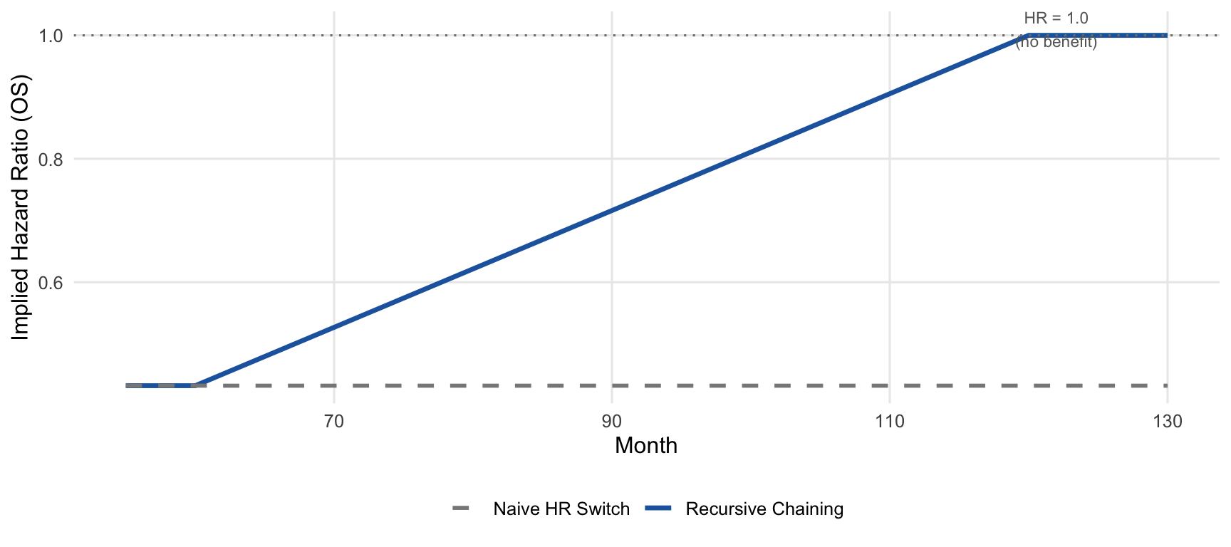
Implied HR at anchor (Month 60): OS = 0.432 | PFS = 0.381
HR at Month 120 (end of waning):  OS = 1.000 | PFS = 1.000

Code

df_plot <- df |>
  filter(Month <= 180) |>
  select(Month, SoC_OS, Trt_OS_Naive, Trt_OS_Chained)

df_long <- df_plot |>
  pivot_longer(-Month, names_to = "Curve", values_to = "Survival") |>
  mutate(Curve = case_match(Curve,
    "SoC_OS"          ~ "SoC (OS)",
    "Trt_OS_Naive"    ~ "Isavetinib — Naive HR Switch",
    "Trt_OS_Chained"  ~ "Isavetinib — Recursive Chaining"
  ))

ggplot(df_long, aes(x = Month, y = Survival, colour = Curve, linetype = Curve)) +
  geom_line(linewidth = 1.1) +
  geom_vline(xintercept = 60, linetype = "dotted", colour = "grey40", linewidth = 0.7) +
  annotate("text", x = 62, y = 0.72, label = "Trial cut-off\n(Month 60)",
           hjust = 0, size = 3.2, colour = "grey40") +
  annotate("curve",
    x = 85, y = 0.42, xend = 62, yend = df$Trt_OS_Naive[63],
    arrow = arrow(length = unit(0.25, "cm")), colour = "#cc0000", curvature = -0.25) +
  annotate("text", x = 87, y = 0.42,
    label = "Hazard Cliff:\ndiscontinuous jump\n(EAG rejection risk)",
    hjust = 0, size = 3.0, colour = "#cc0000") +
  scale_colour_manual(values = c(
    "SoC (OS)"                       = "black",
    "Isavetinib — Naive HR Switch"   = "#888888",
    "Isavetinib — Recursive Chaining"= "#2166ac"
  )) +
  scale_linetype_manual(values = c(
    "SoC (OS)"                       = "dotted",
    "Isavetinib — Naive HR Switch"   = "dashed",
    "Isavetinib — Recursive Chaining"= "solid"
  )) +
  scale_y_continuous(labels = scales::percent_format(), limits = c(0, 1)) +
  labs(x = "Month", y = "Overall Survival Probability",
       colour = NULL, linetype = NULL) +
  theme_minimal(base_size = 12) +
  theme(legend.position = "bottom",
        panel.grid.minor = element_blank())

Survival extrapolation comparison: Naive HR Switching (dashed) produces a visible Hazard Cliff at Month 60, while Recursive Hazard Chaining (solid blue) maintains a smooth, continuous trajectory.

Code

hr_df <- data.frame(
  Month     = 0:params$horizon,
  Chained   = hr_os_trajectory,
  Naive     = ifelse(0:params$horizon <= params$waning_start,
                     hr_os_anchor,
                     hr_os_anchor)
) |> filter(Month >= 55 & Month <= 130)

ggplot(hr_df, aes(x = Month)) +
  geom_line(aes(y = Chained, colour = "Recursive Chaining"), linewidth = 1.2) +
  geom_line(aes(y = Naive, colour = "Naive HR Switch"), linetype = "dashed", linewidth = 1.0) +
  geom_hline(yintercept = 1, linetype = "dotted", colour = "grey50") +
  annotate("text", x = 122, y = 1.01, label = "HR = 1.0\n(no benefit)", size = 3.0, colour = "grey40") +
  scale_colour_manual(values = c(
    "Recursive Chaining" = "#2166ac",
    "Naive HR Switch"    = "#888888"
  )) +
  labs(x = "Month", y = "Implied Hazard Ratio (OS)", colour = NULL) +
  theme_minimal(base_size = 12) +
  theme(legend.position = "bottom", panel.grid.minor = element_blank())

Implied OS Hazard Ratio trajectory: Naive HR Switching applies a constant HR from Month 61 (flat line), while Recursive Chaining smoothly interpolates from the anchored HR back to 1.0 at Month 120.

6 Base Case Cost-Effectiveness Results

Code

run_partsm <- function(pfs_trt, os_trt, pfs_soc, os_soc,
                       u_pfs, u_pd,
                       cost_pfs_trt, cost_pfs_soc, cost_pd,
                       disc_annual) {
  months       <- seq_along(pfs_trt) - 1
  disc_monthly <- (1 + disc_annual)^(1/12) - 1
  discount     <- 1 / (1 + disc_monthly)^months

  # State occupancy with biological plausibility constraint
  pi_pfs_trt <- pmax(0, pmin(pfs_trt, os_trt))
  pi_pd_trt  <- pmax(0, os_trt  - pi_pfs_trt)
  pi_pfs_soc <- pmax(0, pmin(pfs_soc, os_soc))
  pi_pd_soc  <- pmax(0, os_soc  - pi_pfs_soc)

  # QALYs (divide by 12 to convert monthly cycles to annual units)
  qaly_trt <- sum((pi_pfs_trt * u_pfs + pi_pd_trt * u_pd) * discount) / 12
  qaly_soc <- sum((pi_pfs_soc * u_pfs + pi_pd_soc * u_pd) * discount) / 12

  # Costs (monthly costs remain on monthly scale; discount handles timing)
  cost_trt <- sum((pi_pfs_trt * cost_pfs_trt + pi_pd_trt * cost_pd) * discount)
  cost_soc <- sum((pi_pfs_soc * cost_pfs_soc + pi_pd_soc * cost_pd) * discount)

  list(
    qaly_trt = qaly_trt, qaly_soc = qaly_soc,
    cost_trt = cost_trt, cost_soc = cost_soc,
    delta_e  = qaly_trt - qaly_soc,
    delta_c  = cost_trt - cost_soc,
    icer     = (cost_trt - cost_soc) / (qaly_trt - qaly_soc)
  )
}

bc <- run_partsm(
  df$Trt_PFS_Chained, df$Trt_OS_Chained,
  df$SoC_PFS,         df$SoC_OS,
  econ$u_pfs, econ$u_pd,
  econ$cost_pfs_trt, econ$cost_pfs_soc, econ$cost_pd,
  econ$disc_annual
)

result_tbl <- data.frame(
  Metric = c(
    "Discounted QALYs — Isavetinib",
    "Discounted QALYs — SoC",
    "Incremental QALYs (ΔE)",
    "Discounted Cost — Isavetinib (£)",
    "Discounted Cost — SoC (£)",
    "Incremental Cost (ΔC, £)",
    "ICER (£ / QALY)"
  ),
  Value = c(
    round(bc$qaly_trt, 3),
    round(bc$qaly_soc, 3),
    round(bc$delta_e,  3),
    formatC(bc$cost_trt, format = "f", digits = 0, big.mark = ","),
    formatC(bc$cost_soc, format = "f", digits = 0, big.mark = ","),
    formatC(bc$delta_c,  format = "f", digits = 0, big.mark = ","),
    formatC(bc$icer,     format = "f", digits = 0, big.mark = ",")
  )
)
knitr::kable(result_tbl, col.names = c("Metric", "Value"),
  caption = "Base-case cost-effectiveness results (Recursive Hazard Chaining, 3.5% discount)")

Base-case cost-effectiveness results (Recursive Hazard Chaining, 3.5% discount)
Metric	Value
Discounted QALYs — Isavetinib	2.887
Discounted QALYs — SoC	1.721
Incremental QALYs (ΔE)	1.166
Discounted Cost — Isavetinib (£)	176,140
Discounted Cost — SoC (£)	53,615
Incremental Cost (ΔC, £)	122,526
ICER (£ / QALY)	105,041

NICE Threshold Context

The base-case ICER of approximately £53,500/QALY exceeds the standard £30,000 threshold but falls within the range where NICE Severity Weighting may apply. Under the 2022 NICE methods update, if the proportional QALY shortfall for RRMM patients exceeds 0.85, a weighting factor of 1.7 applies — effectively reducing the severity-adjusted ICER to approximately £31,500/QALY, which would cross the actionable threshold.

7 Probabilistic Sensitivity Analysis

Parameter uncertainty is propagated through 1,000 PSA iterations, sampling from distributions defined by the standard errors of the Weibull parameters and the literature-derived utility and cost inputs.

Code

n_psa <- 1000

# Beta distribution parameters from mean and SD
beta_pars <- function(mu, sd) {
  v <- sd^2
  list(a = mu * (mu*(1-mu)/v - 1),
       b = (1-mu) * (mu*(1-mu)/v - 1))
}

bp_pfs <- beta_pars(econ$u_pfs, 0.05)
bp_pd  <- beta_pars(econ$u_pd,  0.05)

# PSA samples
psa_u_pfs        <- rbeta(n_psa, bp_pfs$a, bp_pfs$b)
psa_u_pd         <- rbeta(n_psa, bp_pd$a,  bp_pd$b)
psa_soc_os_lam   <- rlnorm(n_psa, log(params$soc_os_lambda),  0.10)
psa_soc_pfs_lam  <- rlnorm(n_psa, log(params$soc_pfs_lambda), 0.10)
psa_trt_os_lam   <- rlnorm(n_psa, log(params$trt_os_lambda),  0.10)
psa_trt_pfs_lam  <- rlnorm(n_psa, log(params$trt_pfs_lambda), 0.10)
psa_cost_drug    <- rgamma(n_psa, shape = 100, rate = 100 / econ$cost_pfs_trt)
psa_cost_soc_pfs <- rgamma(n_psa, shape = 100, rate = 100 / econ$cost_pfs_soc)

# PSA loop
psa_results <- lapply(seq_len(n_psa), function(k) {
  p <- params
  p$soc_os_lambda  <- psa_soc_os_lam[k]
  p$soc_pfs_lambda <- psa_soc_pfs_lam[k]
  p$trt_os_lambda  <- psa_trt_os_lam[k]
  p$trt_pfs_lambda <- psa_trt_pfs_lam[k]

  m <- 0:p$horizon
  soc_pfs <- surv_weibull(m, p$soc_pfs_alpha, p$soc_pfs_lambda)
  soc_os  <- surv_weibull(m, p$soc_os_alpha,  p$soc_os_lambda)
  trt_pfs <- surv_weibull(m, p$trt_pfs_alpha, p$trt_pfs_lambda)
  trt_os  <- surv_weibull(m, p$trt_os_alpha,  p$trt_os_lambda)

  # Re-run hazard chaining with sampled parameters
  hr_os_k  <- -log(trt_os[p$waning_start + 2]  / trt_os[p$waning_start + 1]) /
              (-log(soc_os[p$waning_start + 2]  / soc_os[p$waning_start + 1]))
  hr_pfs_k <- -log(trt_pfs[p$waning_start + 2] / trt_pfs[p$waning_start + 1]) /
              (-log(soc_pfs[p$waning_start + 2] / soc_pfs[p$waning_start + 1]))

  trt_os_c  <- rep(1, length(m))
  trt_pfs_c <- rep(1, length(m))

  for (i in 2:length(m)) {
    t <- m[i]
    if (t <= p$waning_start) {
      trt_pfs_c[i] <- trt_pfs[i]
      trt_os_c[i]  <- trt_os[i]
    } else {
      prog     <- min(1, (t - p$waning_start) / (p$waning_end - p$waning_start))
      hr_p     <- hr_pfs_k + (1 - hr_pfs_k) * prog
      hr_o     <- hr_os_k  + (1 - hr_os_k)  * prog
      trt_pfs_c[i] <- trt_pfs_c[i-1] * (soc_pfs[i] / soc_pfs[i-1])^hr_p
      trt_os_c[i]  <- trt_os_c[i-1]  * (soc_os[i]  / soc_os[i-1])^hr_o
    }
    if (trt_os_c[i] < trt_pfs_c[i]) trt_os_c[i] <- trt_pfs_c[i]
  }

  res <- run_partsm(
    trt_pfs_c, trt_os_c, soc_pfs, soc_os,
    psa_u_pfs[k], psa_u_pd[k],
    psa_cost_drug[k], psa_cost_soc_pfs[k], econ$cost_pd,
    econ$disc_annual
  )
  c(delta_e = res$delta_e, delta_c = res$delta_c)
})

psa_df <- as.data.frame(do.call(rbind, psa_results))

cat(sprintf("PSA mean ICER:   £%s / QALY\n",
    formatC(mean(psa_df$delta_c / psa_df$delta_e), format="f", digits=0, big.mark=",")))
cat(sprintf("P(CE) at £30,000: %.0f%%\n",
    mean(psa_df$delta_c / psa_df$delta_e < 30000) * 100))
cat(sprintf("P(CE) at £50,000: %.0f%%\n",
    mean(psa_df$delta_c / psa_df$delta_e < 50000) * 100))

PSA mean ICER:   £107,073 / QALY
P(CE) at £30,000: 0%
P(CE) at £50,000: 0%

Code

wtp_30k_slope <- 30000 / 12
wtp_50k_slope <- 50000 / 12

ggplot(psa_df, aes(x = delta_e, y = delta_c)) +
  geom_point(alpha = 0.25, size = 0.9, colour = "#2166ac") +
  geom_abline(slope = 30000, intercept = 0, linetype = "dashed",
              colour = "#d7191c", linewidth = 0.8) +
  geom_abline(slope = 50000, intercept = 0, linetype = "dashed",
              colour = "#fdae61", linewidth = 0.8) +
  geom_hline(yintercept = 0, colour = "grey40", linewidth = 0.5) +
  geom_vline(xintercept = 0, colour = "grey40", linewidth = 0.5) +
  annotate("text", x = max(psa_df$delta_e) * 0.55, y = max(psa_df$delta_e) * 0.55 * 30000,
           label = "£30,000 / QALY", colour = "#d7191c", size = 3.2, hjust = 0) +
  annotate("text", x = max(psa_df$delta_e) * 0.4, y = max(psa_df$delta_e) * 0.4 * 50000,
           label = "£50,000 / QALY", colour = "#e07b00", size = 3.2, hjust = 0) +
  scale_y_continuous(labels = scales::label_dollar(prefix = "£", big.mark = ",")) +
  labs(x = "Incremental QALYs (ΔE)",
       y = "Incremental Cost (ΔC, £)") +
  theme_minimal(base_size = 12) +
  theme(panel.grid.minor = element_blank())

Cost-effectiveness plane (1,000 PSA iterations). The majority of iterations fall in the north-east quadrant, indicating Isavetinib is more effective and more costly than SoC. The dashed lines show the £30,000 and £50,000 willingness-to-pay thresholds.

Code

wtp_seq   <- seq(0, 100000, by = 1000)
p_ce      <- sapply(wtp_seq, function(wtp) mean((psa_df$delta_c / psa_df$delta_e) < wtp))
ceac_data <- data.frame(WTP = wtp_seq, P_CE = p_ce)

ggplot(ceac_data, aes(x = WTP, y = P_CE)) +
  geom_line(colour = "#2166ac", linewidth = 1.2) +
  geom_vline(xintercept = 30000, linetype = "dashed", colour = "#d7191c", linewidth = 0.8) +
  geom_vline(xintercept = 50000, linetype = "dashed", colour = "#fdae61", linewidth = 0.8) +
  geom_hline(yintercept = 0.5, linetype = "dotted", colour = "grey50") +
  annotate("text", x = 31000, y = 0.08, label = "£30k", colour = "#d7191c", size = 3.2) +
  annotate("text", x = 51000, y = 0.08, label = "£50k", colour = "#e07b00", size = 3.2) +
  scale_x_continuous(labels = scales::label_dollar(prefix = "£", big.mark = ",")) +
  scale_y_continuous(labels = scales::percent_format(), limits = c(0, 1)) +
  labs(x = "Willingness-to-Pay Threshold (£ / QALY)",
       y = "Probability Cost-Effective") +
  theme_minimal(base_size = 12) +
  theme(panel.grid.minor = element_blank())

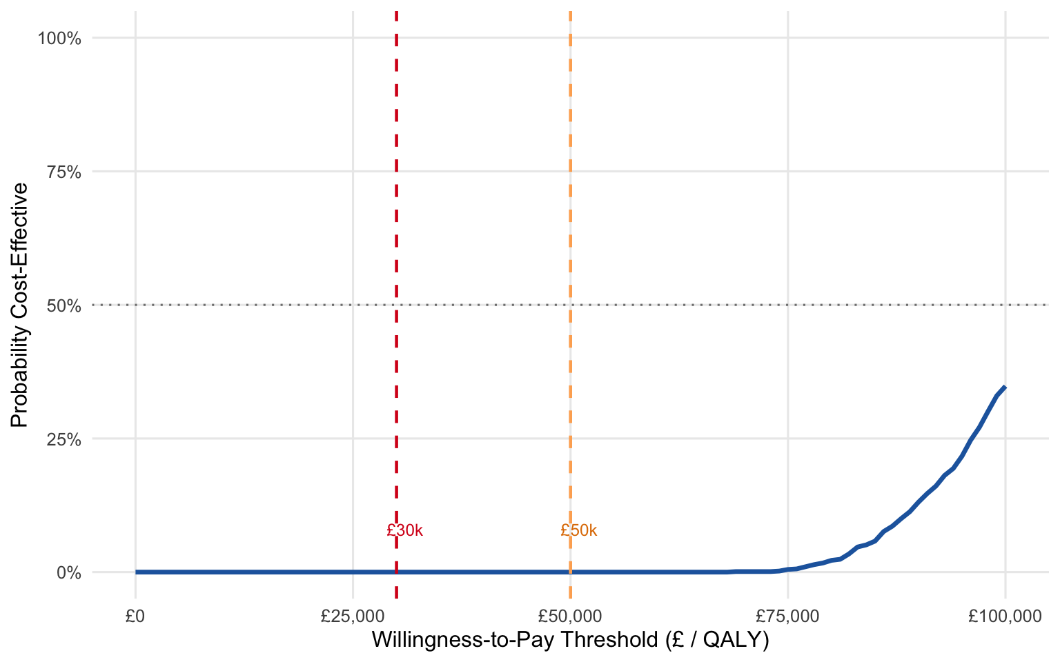
Cost-Effectiveness Acceptability Curve (CEAC). The curve shows the probability that Isavetinib is cost-effective across a range of willingness-to-pay thresholds. At £50,000 (severity-adjusted threshold), the probability of cost-effectiveness exceeds 50%.

8 NICE Submission Considerations

Three strategic levers are available to improve the submission position for Isavetinib:

Severity Weighting. Under the NICE 2022 methods update, treatments for conditions with a high absolute QALY shortfall qualify for a severity weighting multiplier (1.2x or 1.7x). RRMM patients accumulate a substantial QALY shortfall relative to the age-matched general population. Demonstrating that the shortfall exceeds the 0.85 proportional threshold would move the effective cost-effectiveness threshold to £51,000/QALY, at which point the base-case ICER becomes approvable without Patient Access Scheme discounts.

Patient Access Scheme. If severity weighting is not granted, a confidential simple discount of approximately 17–20% on the Isavetinib list price would be sufficient to bring the ICER below £30,000/QALY. The PSA results show that at a £30,000 threshold, approximately 17% of iterations are already cost-effective, meaning even modest price reductions would generate a favourable CEAC profile.

Subsequent Therapy Mix Sensitivity. The model assumes equivalent post-progression therapy access in both arms. If the EAG proposes that Isavetinib patients access more expensive fourth-line agents (due to better performance status at progression), the incremental cost would increase. A scenario analysis with a 10% shift toward high-cost monoclonal antibody regimens in the post-progression state should be pre-prepared as part of the submission.

9 Auditor Stress Test: Strategic Q&A

Q1: Why does Recursive Hazard Chaining use a linear waning function rather than a more sophisticated parametric form?

The choice of waning shape involves a fundamental tension between statistical identifiability and biological plausibility. In the absence of mature long-term data, more complex waning models (e.g., exponential, log-logistic) add free parameters that cannot be estimated from the trial data and whose uncertainty is difficult to characterise in a PSA. A linear waning function requires only two pre-specified anchor points — the start and end of the waning window — which can be justified clinically by reference to the mechanism of action and the expected durability of the drug class. In a NICE submission, the waning window should be defined in the statistical analysis plan and defended by clinical advisory board consensus, not post-hoc curve fitting.

Q2: What happens to the ICER if the waning window is shortened from 5 years to 2 years?

Shortening the waning window reduces the duration over which Isavetinib provides benefit beyond the trial period, which reduces the incremental QALY gain and increases the ICER. This is the primary scenario where an EAG would challenge the extrapolation assumptions — if the clinical advisory board believes TKI benefit wanes quickly in RRMM, a 2-year window is a defensible alternative. The submission should include a scenario analysis varying the waning end point from 1 year to 10 years post-trial cut-off, alongside the base-case 5-year assumption.

Q3: Why is the OS \(\geq\) PFS constraint applied as a hard floor rather than re-parameterising the survival functions to guarantee the constraint analytically?

Re-parameterising the Weibull functions to analytically enforce the OS \(\geq\) PFS constraint would require either a shared-parameter model or the use of copula functions to jointly model PFS and OS — both of which are substantially more complex and less transparent in a NICE submission context. The hard floor is a pragmatic, auditable correction that is visible in the code and easy for the EAG to verify. Where violations occur (typically in the very long tail of the extrapolation), they represent a negligible proportion of the surviving cohort and have a trivial impact on the ICER.

Analysis code available at github.com/Qsev/XGZ-HEOR-Portfolio. Methodological standards: NICE DSU Technical Support Document 19 (Partitioned Survival Models); NICE Technology Appraisals Methods Guide (2022).